1. Self-Organizing Maps Projection of p dimensional observations to a two (or one) dimensional grid space Constraint version of K-means clustering –Prototypes lie in a one- or two-dimensional manifold (constrained topological map; Teuvo Kohonen, 1993) K prototypes: Rectangular grid, hexagonal grid Integer pair l j  Q 1 x Q 2, where Q 1 =1, …, q 1 & Q 2 =1,…,q 2 (K = q 1 x q 2 ) High-dimensional observations projected to the two- dimensional coordinate system

3. SOM Algorithm Prototype m j, j =1, …, K, are initialized Each observation x i is processed one at a time to find the closest prototype m j in Euclidean distance in the p-dimensional space All neighbors of m j, say m k, move toward x i as m k  m k +  x i – m k  Neighbors are all m k such that the distance between m j and m k are smaller than a threshold r (neighbor includes itself) –Distance defined on Q 1 x Q 2, not on the p-dimensional space SOM performance depends on learning rate  and threshold r –Typically,  and r are decreased from 1 to 0 and from R (predefined value) to 1 at each iteration over, say, 3000 iterations

6. SOM properties If r is small enough, each neighbor contains only one point  spatial connection between prototypes is lost  converges at a local minima of K-means clustering Need to check the constraint reasonable: compute and compare reconstruction error  =||x-m|| 2 for both methods (SOM’s  is bigger, but should be similar)

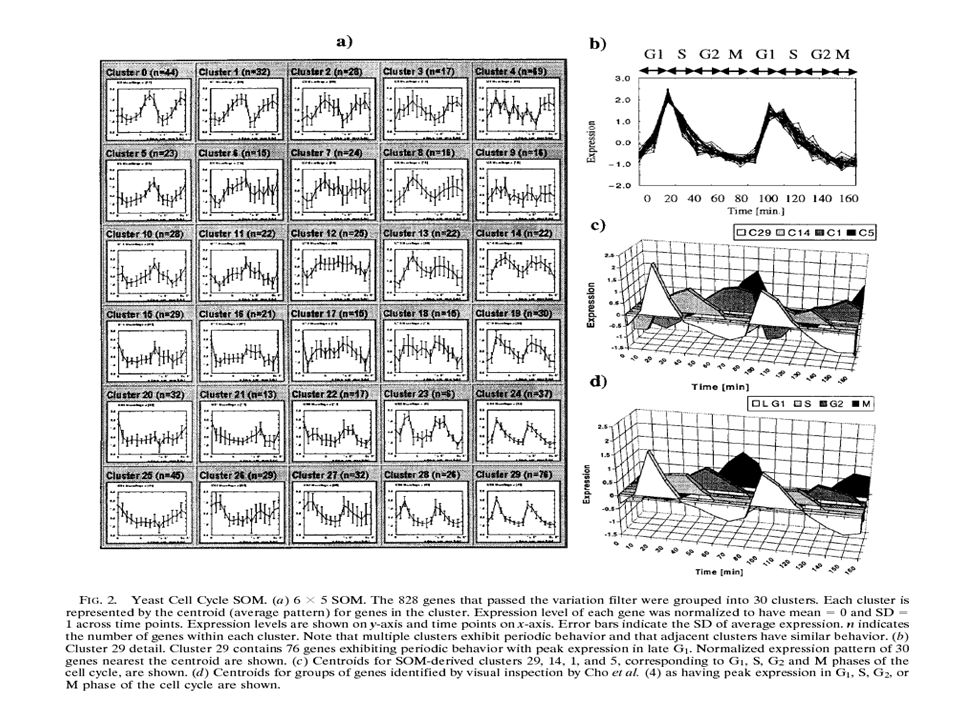
8. Tamayo et al. (1999; GeneCluster) Self-organizing maps (SOM) on microarray data - Hematopoietic cell lines (HL60, U937, Jurkat, and NB4): 4x3 SOM - Yeast data in Eisen et al. reanalyzed by 6x5 SOM

10. Principal Component Analysis Data x i, i=1,…,n, are from the p-dimensional space (n  p) –Data matrix: Xn x p Singular decomposition X = U  V T, where –  is a non-negative diagonal matrix with decreasing diagonal entries of eigen values (or singular value) i, –Un x p with orthogonal columns (u i t u j = 1 if i  j, =0 if i=j), and –Vp x p is an orthogonal matrix The principal components are the columns of XV (=U  –X and V have the same rank, at most p of non-zero eigen values

13. PCA properties The first column of XV or DU is the 1 st principal component, which represents the direction with the largest variance (the first eigen value represents its magnitude) The second column is for the second largest variance uncorrelated with the first, and so on. The first q columns, q < p, of XV are the linear projection of X into q diensions with the largest variance Let x = U  q V T, where  q is the diagonal matrix of  with q non-zero diagonals  x is best possible approximate of X with rank q

14. Traditional PCA Variance-Covariance matrix S from data X n x p –Eigen value decomposition: S = CDC T, with C an orthogonal matrix –(n-1)S = X T X = (U  V T)T U  V T = V  U T U  V T = V  2 V T –Thus, D =     n-1) and  C = V

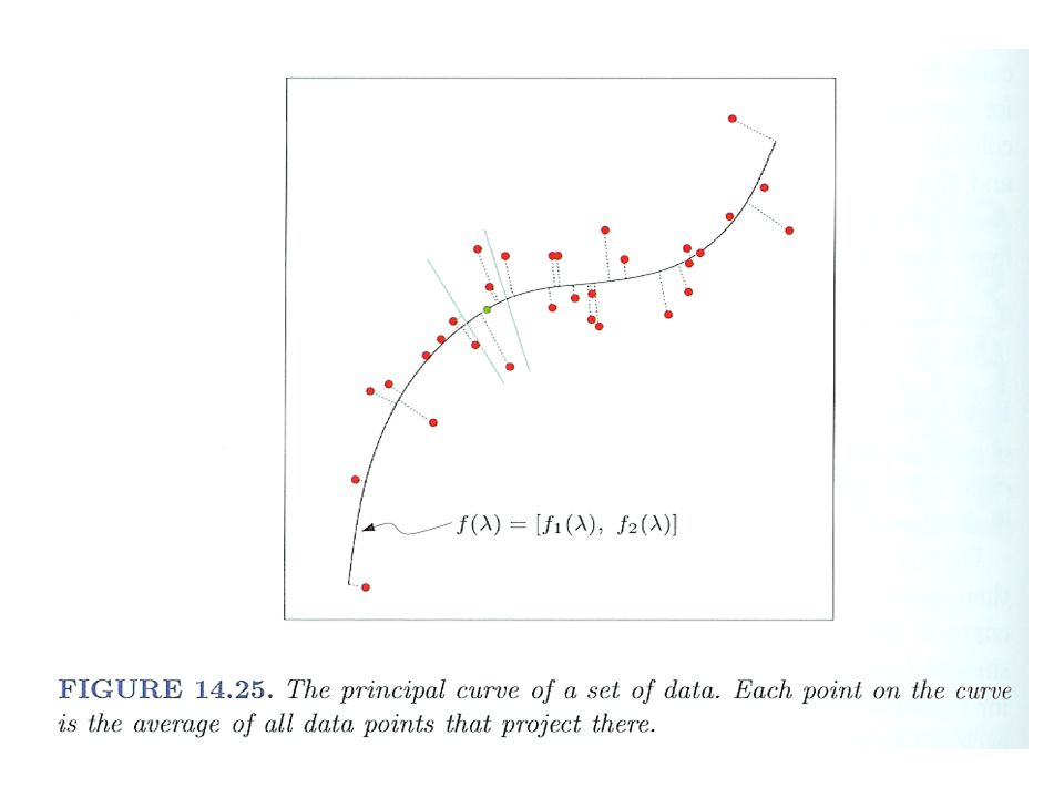
15. Principal Curves and Surfaces Let f( ) be a parameterized smooth curve on the p- dimensional space For data x, let f (x) define the closest point on the curve to x Then f( ) is the principal curve for random vector X, if f( ) = E[X| f (X) = ] Thus, f( ) is the average of all data points that project to it

17. Algorithm for finding the principal curve Let f( ) have its coordinate f( ) = [f 1 ( ), f 2 ( ), …, f p ( )] where random vector X = [X 1, X 2, …, X p ] Then iterate the following alternating steps until converge: –(a) f j ( )  E[X j | (X) = l], j =1, …, p –(b) f (x)  argmin  ||x – f( )|| 2 The solution is the principal curve for the distribution of X

19. Multidimensional scaling (MDS) Observations x 1, x 2, …, x n in the p-dimensional space with all pair-wise distances (or dissimilarity measure) d ij MDS tries to preserve the structure of the original pair- wise distances as much as possible Then, seek the vectors z 1, z 2, …, z n in the k-dimensional space (k << p) by minimizing “stress function” –S D (z 1,…,z n ) =  i  j [(d ij - ||z i – z j ||) 2 ] 1/2 –Kruskal-Shephard scaling (or least squares) –A gradient descent algorithm is used to find the solution

20. Other MDS approaches Sammon mapping minimizes –  i  j [(d ij - ||z i – z j ||) 2 ] / d ij Classical scaling is based on similarity measure s ij –Often inner product s ij = is used –Then, minimize  i  j [(s ij - ) 2 ]