1. Nikolaj Bjørner Microsoft Research Lecture 5

2. DayTopicsLab 1Overview of SMT and applications. SAT solving part I. Program exploration with Pex 2SAT solving part II. Congruence closure Encoding combinatorial problems 3Combining solvers. A solver for arithmetic. Encoding arithmetic problems 4Solvers for Bit-vectors, arrays, data-types, and other theories Build your own solver 5Solvers part II. Extended topics: Pattern matching Program verification with Spec#/Boogie

3. Array decision procedures (part 2) Quantifiers and SMT solvers Lab: Build your own theory decision procedure on top of Z3

5. Functions:  F = { read, write } Predicates:  P = { = } Convention a[i] means: read(a,i) Non-extensional arrays T A :  a, i, v. write(a,i,v)[i] = v  a, i, j, v. i  j  write(a,i,v)[j] = a[j] Extensional arrays: T EA = T A +  a, b. ((  i. a[i] = b[i])  a = b)

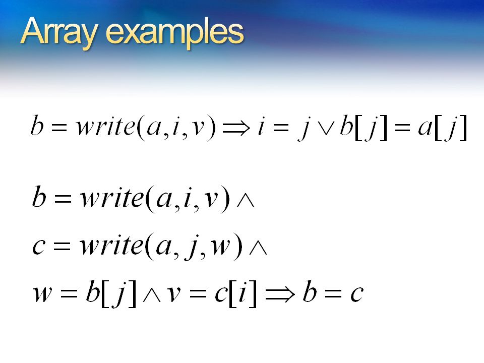
7. Is valid Is unsat (array axiom) Is unsat (congruence)

8. Is valid Is unsat

9. Array axiom

10. Is unsat

11. Case:

12. Array axiom

13. Case:

14. Congruence

15. Case:

17. Extensionality

18. Case: Extensionality

19. Case: Skolemize

20. Case: Array axiom

21. Case:

22. Let L be literals over  F = { read, write } Find M such that: M ⊨ T A L Basic algorithm, reduce to E: for every sub-term read(a,i), write(b,j,v) in L i  j  a = b  read(write(b,j,v),i) = read(a,i) read(write(b,j,v),j) = v Find M E, such that M E ⊨ E L  AssertedAxioms

23. Correctness of basic algorithm: M E satisfies array axioms on terms in L. To show that M E can be extended to model for arrays: From Congurence Closure C * build model: a M = [| * d1  * r1, * d2  * r2, * d3 .., else  v root(a) |] Where read M (a M, * di ) = * r1 e.g., * r1 = root(read(root(a),root(i)) under C * Model satisfies array axioms. For every write(a,i,v) the model satisfies write(a,i,v)[j] = a[j] whenever i M  j M (first axiom) and also write(a,i,v)[i] = v (second axiom). v root(a) was added to make arrays different unless they were forced to be (no extensionality)

24. A non-theorem a and b need not be equal even if the array axioms hold.

25. To enforce:  a, b. ((  i. a[i]= b[i])  a = b) For every pair a, b in L, Add fresh constant i ab Add axiom a  b  a[i ab ]  b[i ab ]

26. Arrays may be more than just read/write. The constant array:  v, i. const(v)[i] = v Generalized write:  a,b,c, i. a[i] = b[i]  write  (a,b,c)[i] = c[i]  a,b,c, i. a[i]  b[i]  write  (a,b,c)[i] = b[i] We now have sets:  = const(false), T = const(true), A  B = write  ( ,A,B)[i] A  B = write  (T,A,B)[i] Ranges:  l,u, x. range(l,u)[x]  l  x  u

27. Claim: Same kind of reduction to E (and arithmetic) works Integer ranges, require slightly more  range(l,u)[l-1],  range(l,u)[u+1] range(l,u)[l], range(l,u)[u] Is there a general principle underpinning such extensions?

28. Consider a more general formulation.  is a conjunction of: Equalities, disequalities  i, j, k. G(i,j,k)  F(i,j,k) Where G is a guard formula comparing indices: And-or formula of i  j, i  c Claim: We can always eliminate i =j from the guard. Where F is a general formula with arrays, Restriction: no nested array formulas. Example:  j. if i = j then b[i] = v else b[i] = a[i] Encodes that b = write(a,i,v)

29.  i, j, k. G(i,j,k)  F(i,j,k) Where G is a guard formula comparing indices: And-or formula of i  j, i  c Claim: We can always eliminate i =j or i = c from the guard.  i, j, k. i = j  k  c  j  c’  F(i,j,k)   i, k. k  c  i  c  F(i,i,k)

30.  i, j, k. G(i,j,k)  F(i,j,k) Where G is a guard formula comparing indices: And-or formula of i  j, i  c Claim: We can always or from the guard  i, j, k. G(i,j,k)  G’(i,j,k)  F(i,j,k)   i, j, k. G(i,j,k)  F(i,j,k)  i, j, k. G’(i,j,k)  F(i,j,k)

31.  i, j, k. G(i,j,k)  F(i,j,k) Where G is conjunction of i  j, i  c Decision procedure: Collect all c, where a[c] or c = i Instantiate quantifiers by all combinations of such indices. Check for E – satisfiability of ground formula. Correctness: All quantified formulas are satisfied by C *.

32.  i, j, k. G(i,j,k)  F(i,j,k) Where G is conjunction of i c Decision procedure: Collect all c, where a[c], c i occurs in formula. For each c, also add c-1, c+1 to collection. Instantiate quantifiers by all combinations of collected indices. Check for ILA + E – satisfiability of ground formula.

34. Bit-vectors Algebraic data-types Queues Partial orders Binary relations Heaps (reachability)

36. Checking the validity of  in a theory T:  is T-valid  T-unsat:   T-unsat:  x  y  z  u.  (prenex of  )  T-unsat:  x  z.  [f(x),g(x,z)] (skolemize)  T-unsat:  [f(a 1 ),g(a 1,b 1 )]  … (instantiate)   [f(a n ),g(a n,b n )] (  if compactness )  T-unsat:  1  …   m (DNF) where each  i is a conjunction.

37. We can use DPLL(T) for  with quantifiers. Treat quantified sub-formulas as atomic predicates. In other words, if  x.  (x) is a sub-formula if , then introduce fresh p. Solve instead  [  x.  (x)  p]

38. Suppose DPLL(T) sets p to false  any model M for  must satisfy: M ⊨   x.  (x)  for some sk x : M ⊨   (sk x ) In general: ⊨  p    (sk x )

39. Suppose DPLL(T) sets p to true  any model M for  must satisfy: M ⊨  x.  (x)  for every term t: M ⊨  (t) In general: ⊨ p   (t) For every term t.

40. Summary of auxiliary axioms: ⊨  p    (sk x )For fixed, fresh sk x ⊨ p   (t) For every term t. Which terms t to use for auxiliary axioms of the second kind?

41. ⊨ p   (t) For every term t. Approach: Add patterns to quantifiers Search for instantiations in E-graph.  a,i,v { write(a,i,v) }. read(write(a,i,v),i) = v

42. ⊨ p   (t) For every term t. Approach: Add patterns to quantifiers Search for pattern matches in E-graph.  a,i,v { write(a,i,v) }. read(write(a,i,v),i) = v Add equality every time there is a write(b,j,w) term in E.

43. Array example  a,i,v { write(a,i,v) }. write(a,i,v)[i] = v Add equality every time there is a write(b,j,w) term in E.  a,i,j,v { write(a,i,v)[j] }. i  j  write(a,i,v)[j]=a[j] Add implication every time there is a read of a write.  a,i,j,v { write(a,i,v), a[j] }. i  j  write(a,i,v)[j]=a[j] Add implication every time there is both a write and a read of a.

44. Input A set of ground equations E a ground term t and a pattern pat, with variables. Output The set of substitutions  modulo E over the variables in pat, such that E  ╞ t =  (pat)

45. Given:  A,I,J,V { write(A,I,V), A[J] }. I  J  write(A,I,V)[J]=A[J] E = { g(a) = f(b, c), b = d, a = c } Match: E  ╞ write(g(c),2,1) =  (write(A,I,V)), f(d,a)[4] =  (A[J]) For  = [ A  g(c), I  2, V  1, J  4 ]

46. Review: Standard matching match(t, X,  ) =   [ X  t] if X  dom(  ) match(t, X,  ) =  if  (X) = t match(t, X,  ) = fail if  (X)  t match(t, t,  ) =  match( f(..), g(..),  ) = fail match(f(t 1,..,t n ), f(pat 1,..,pat n ),  ) = match(t 1,pat 1, … match(t n, pat n,  ))

47. E-matching generalizes standard matching: Every term t can be congruent to a set of other terms class(t) = {t 1,..,t n } in the E-graph. Each congruent term is tried. Terms are equal if they are in the same class. find(t) is the equivalence class root. t and t’ are equal if: find(t) = find(t’)

48. E-graph: Term: Pattern:

50. E-matching is in theory NP-hard The real challenge is finding new matches Incrementally during a backtracking search In a large database of patterns, many sharing substantial structure [de Moura & Bjørner CADE 2007]

51. Match is invoked for every pattern in database. To avoid common work: Compile set of patterns into instructions. By partial evaluation of naïve algorithm Instruction sequences share common sub- terms. Substitutions are stored in registers, backtracking just updates the registers.

52. pat1: write(A,I,V)[I] Pattern Instructions(pat1)Instructions(pat1) Specialize Term

53. pat2: write(A,I,V) Pattern Instructions(pat1)Instructions(pat1) Specialize Instructions(pat2)Instructions(pat2) Term

54. pat2: write(A,I,V) Pattern Specialize Instructions(pat1+pat2)Instructions(pat1+pat2) Term

55. Pattern f(x 1, g(x 1, a), h(x 2 ), b): PcInstructions pc0init(f, pc1) pc1check(4, b, pc2) Pc2bind(2, g, 5, pc3) Pc3compare(1, 5, pc4) Pc4check(6, a, pc5) Pc5bind(3, h, 7, pc6) Pc6yield(1,7) Instructionf(h(a),g(h(c),a),h(c), b) init(f) reg[1]  h(a), reg[2]  g(h(c),a), reg[3]  h(c), reg[4]  b  check(4, b)reg[4] = b  bind(2, g, 5) reg[5]  h(c), reg[6]  a  compare(1, 5) h(a) = reg[1]  reg[5] = h(c) 

56. Pattern f(x 1, g(x 1, a), h(x 2 ), b): PcInstructions pc0init(f, pc1) pc1check(4, b, pc2) Pc2bind(2, g, 5, pc3) Pc3compare(1, 5, pc4) Pc4check(6, a, pc5) Pc5bind(3, h, 7, pc6) Pc6yield(1,7) Instructionf(h(a),g(h(a),a),h(c), b) init(f) reg[1]  h(a), reg[2]  g(h(a),a), reg[3]  h(c), reg[4]  b  check(4, b)reg[4] = b  bind(2, g, 5) reg[5]  h(a), reg[6]  a  compare(1, 5) h(a) = reg[1] =reg[5] = h(a)  check(6, a)a = reg[6] = a  bind(3, h, 7) reg[7]  c  yield(1,7) X 1  h(a), X 2  c 

57. First execute init: pc: init(f, pc’) - match term f(t 1,.. t n ) store t 1,.., t n into reg[1],..,reg[n]. goto pc’ If pattern is a ground term: pc: check(i, t, pc’) – check that reg[i] = t, on success goto pc’ on failure goto backtrack For repeated variables in pattern: pc: compare(i, j, pc’) – check that reg[i] = reg[j], on success goto pc’ on failure goto backtrack

58. pc: bind(i, f, o, pc’) – for each term f(t 1,.. t n ) in reg[i] do store t 1,.., t n into reg[o],..,reg[o+n-1]. goto pc’ pc: choose(pc’’,pc’) - first go to pc’ and perform matching then go to pc’’ and perform matching pc: yield(i 1,…,i k ) – produce substitution x 1  reg[x 1 ],.., x k  reg[i k ]

60. Forward pruning Prune exponential search early on f(g(x,y), h(x,z)) – first check that t 1 = g(…) and t 2 = h(…) when matching f(t 1, t 2 ) Multi-patterns Continue Join = continue + compare

61. 5 = read(b, 2)E 1 = { {5, read(b,2)}, {b} } c = write(a, 2, 4)E 2 = E 1  { {c, write(a,2,4) } b = cE 3 = { {b, c, write(a,2,4)}, {5, read(b,2)} } E 3 ╞ 5 = read(b,2) = read(write(a,2,4),2) Observation: pattern read(write(x, i, v), i) gets enabled when child of read is merged with term labeled by write.

62. Index all patterns with f(…g(…)…) sub-term, that may become enabled when merge(n 1, n 2 ) where  parent p 1 of n 1. Label(p 1 ) = f(…n 1 …)  sibling m 2 of n 2. Label(m 2 ) = g(…)

64. Lazy Instantiation: Have SAT core assign all Boolean variables. Then find new quantifier instantiations. Useful if most instantiations are useless and explode the search space. Eager Instantiation: Find new quantifier instantiations whenever new terms are created and new equalities are asserted. Useful if instantiations help pruning the search space. Hybrid: Uses scoring on useful quantifiers to promote/demote instantiation time.

65. E-matching needs ground (seed) terms. It fails to prove simple properties when ground (seed) terms are not available. Example: ( ∀ x. f(x) ≤ 0) ∧ ( ∀ x. f(x) > 0) Matching loops: ( ∀ x. f(x) = g(f(x))) ∧ ( ∀ x. g(x) = f(g(x))) Inefficiency and/or non-termination. Some solvers have support for detecting matching loops based on instantiation chain length. Our technology for inferring patterns is weak. Strong reliance on (Spec#/Boogie) compiler or theory supplied patterns.

66. Matching-time significantly reduced for DPLL(T) search when using E-matching code trees and inverted path indices. Inverted path indices: Pay for what you use, not for what you might. Lazy vs. Eager depends on quality of patterns.

67. DPLL(QT) is (blatantly) incomplete. E-matching is a heuristic. Saturation calculi offer a strong (and in principle complete) alternative. Plug: Engineering DPLL(T) + Saturation. [de Moura & Bjørner IJCAR 2008]

70. Bradley & Manna: The Calculus of Computation Kroening & Strichman: Decision Procedures An Algorithmic Point of View

71. Http://research.microsoft.com/projects/z3 http://smt-lib.org http://wiki.org/smt Some SMT solvers: Barcelogic, CVC3, Mathsat, Yices

72. [Ack54] W. Ackermann. Solvable cases of the decision problem. Studies in Logic and the Foundation of Mathematics, 1954 [ABC+02] G. Audemard, P. Bertoli, A. Cimatti, A. Kornilowicz, and R. Sebastiani. A SAT based approach for solving formulas over boolean and linear mathematical propositions. In Proc. of CADE’02, 2002 [BDS00] C. Barrett, D. Dill, and A. Stump. A framework for cooperating decision procedures. In 17th International Conference on Computer-Aided Deduction, volume 1831 of Lecture Notes in Artificial Intelligence, pages 79–97. Springer-Verlag, 2000 [BdMS05] C. Barrett, L. de Moura, and A. Stump. SMT-COMP: Satisfiability Modulo Theories Competition. In Int. Conference on Computer Aided Verification (CAV’05), pages 20–23. Springer, 2005 [BDS02] C. Barrett, D. Dill, and A. Stump. Checking satisfiability of first-order formulas by incremental translation to SAT. In Ed Brinksma and Kim Guldstrand Larsen, editors, Proceedings of the 14th International Conference on Computer Aided Verification (CAV ’02), volume 2404 of Lecture Notes in Computer Science, pages 236–249. Springer-Verlag, July 2002. Copenhagen, Denmark [BBC+05] M. Bozzano, R. Bruttomesso, A. Cimatti, T. Junttila, P. van Rossum, S. Ranise, and R. Sebastiani. Efficient satisfiability modulo theories via delayed theory combination. In Int. Conf. on Computer-Aided Verification (CAV), volume 3576 of LNCS. Springer, 2005 [Chv83] V. Chvatal. Linear Programming. W. H. Freeman, 1983

73. [CG96] B. Cherkassky and A. Goldberg. Negative-cycle detection algorithms. In European Symposium on Algorithms, pages 349–363, 1996 [DLL62] M. Davis, G. Logemann, and D. Loveland. A machine program for theorem proving. Communications of the ACM, 5(7):394–397, July 1962 [DNS03] D. Detlefs, G. Nelson, and J. B. Saxe. Simplify: A theorem prover for program checking. Technical Report HPL-2003-148, HP Labs, 2003 [DST80] P. J. Downey, R. Sethi, and R. E. Tarjan. Variations on the Common Subexpression Problem. Journal of the Association for Computing Machinery, 27(4):758–771, 1980 [dMR02] L. de Moura and H. Rueß. Lemmas on demand for satisfiability solvers. In Proceedings of the Fifth International Symposium on the Theory and Applications of Satisfiability Testing (SAT 2002). Cincinnati, Ohio, 2002 [dMB07] L. de Moura and N. Bjørner. Model-based Theory Combination (SMT 2007) [dMB07] L. de Moura and N. Bjørner. Efficient E-matching for SMT solvers (CADE 2007) [dMB08] L. de Moura and N. Bjørner. Z3: An Efficient SMT Solver (TACAS 2008) [DdM06] B. Dutertre and L. de Moura. Integrating simplex with DPLL(T). Technical report, CSL, SRI International, 2006 [GHN+04] H. Ganzinger, G. Hagen, R. Nieuwenhuis, A. Oliveras, and C. Tinelli. DPLL(T): Fast decision procedures. In R. Alur and D. Peled, editors, Int. Conference on Computer Aided Verification (CAV 04), volume 3114 of LNCS, pages 175–188. Springer, 2004

74. [MSS96] J. Marques-Silva and K. A. Sakallah. GRASP - A New Search Algorithm for Satisfiability. In Proc. of ICCAD’96, 1996 [NO79] G. Nelson and D. C. Oppen. Simplification by cooperating decision procedures. ACM Transactions on Programming Languages and Systems, 1(2):245–257, 1979 [NO05] R. Nieuwenhuis and A. Oliveras. DPLL(T) with exhaustive theory propagation and its application to difference logic. In Int. Conference on Computer Aided Verification (CAV’05), pages 321–334. Springer, 2005 [Opp80] D. Oppen. Reasoning about recursively defined data structures. J. ACM, 27(3):403–411, 1980 [PRSS99] A. Pnueli, Y. Rodeh, O. Shtrichman, and M. Siegel. Deciding equality formulas by small domains instantiations. Lecture Notes in Computer Science, 1633:455–469, 1999 [Pug92] William Pugh. The Omega test: a fast and practical integer programming algorithm for dependence analysis. In Communications of the ACM, volume 8, pages 102–114, August 1992 [RT03] S. Ranise and C. Tinelli. The smt-lib format: An initial proposal. In Proceedings of the 1st International Workshop on Pragmatics of Decision Procedures in Automated Reasoning (PDPAR’03), Miami, Florida, pages 94–111, 2003

75. [RS01] H. Ruess and N. Shankar. Deconstructing shostak. In 16th Annual IEEE Symposium on Logic in Computer Science, pages 19–28, June 2001 [SLB03] S. Seshia, S. Lahiri, and R. Bryant. A hybrid SAT-based decision procedure for separation logic with uninterpreted functions. In Proc. 40th Design Automation Conference, pages 425–430. ACM Press, 2003 [Sho81] R. Shostak. Deciding linear inequalities by computing loop residues. Journal of the ACM, 28(4):769–779, October 1981