1. Quantum One: Lecture 7

3. The General Formalism of Quantum Mechanics

4. The General Formalism of Quantum Mechanics Postulate One

5. In the last lecture, we completed our review of Schrödinger's wave mechanics for a free quantum particle, by completing our solution to the initial value problem, which we summarize below. For a free particle described by an initial real space wave function 1.Compute the initial momentum space wave function so that 1.Then, evolve the state of the system, as

6. We also observed that, even when the particle is not free, i.e., when it is acted upon by forces, we can still, at any instant, expand the system in momentum eigenfunctions in terms of a momentum space wave function so that predictions of measurements of momentum can be made based upon the probability density

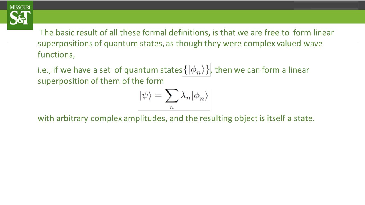
7. We concluded with the observation, that there actually appears to be many ways to represent the dynamical state of this quantum mechanical system. In this lecture, we therefore begin a presentation of the postulates of quantum mechanics in a form that is 1.Manifestly representation independent (but which allows for the natural emergence of appropriate numerical representations), and which 2.In principle applies to arbitrary quantum mechanical systems. One of our goals in going forward is also to provide an appropriate mathematical framework for understanding the content of the more generally formulated postulates.

8. We concluded with the observation, that there actually appears to be many ways to represent the dynamical state of this quantum mechanical system. In this lecture, we therefore begin a presentation of the postulates of quantum mechanics in a form that is 1.Manifestly representation independent (but which allows for the natural emergence of appropriate numerical representations), and which 2.In principle applies to arbitrary quantum mechanical systems. One of our goals in going forward is also to provide an appropriate mathematical framework for understanding the content of the more generally formulated postulates.

9. We concluded with the observation, that there actually appears to be many ways to represent the dynamical state of this quantum mechanical system. In this lecture, we therefore begin a presentation of the postulates of quantum mechanics in a form that is 1.Manifestly representation independent (but which allows for the natural emergence of appropriate numerical representations), and which 2.In principle applies to arbitrary quantum mechanical systems. One of our goals in going forward is also to provide an appropriate mathematical framework for understanding the content of the more generally formulated postulates.

10. We concluded with the observation, that there actually appears to be many ways to represent the dynamical state of this quantum mechanical system. In this lecture, we therefore begin a presentation of the postulates of quantum mechanics in a form that is 1.Manifestly representation independent (but which allows for the natural emergence of appropriate numerical representations), and which 2.In principle applies to arbitrary quantum mechanical systems. One of our goals in going forward is also to provide an appropriate mathematical framework for understanding the content of the more generally formulated postulates.

11. We concluded with the observation, that there actually appears to be many ways to represent the dynamical state of this quantum mechanical system. In this lecture, we therefore begin a presentation of the postulates of quantum mechanics in a form that is 1.Manifestly representation independent (but which allows for the natural emergence of appropriate numerical representations), and which 2.In principle applies to arbitrary quantum mechanical systems. One of our goals in going forward is also to provide an appropriate mathematical framework for understanding the content of the more generally formulated postulates.

12. To this end it is useful to adopt an approach which mixes these two tasks. Thus, we start out by simply stating the first postulate, and then follow this statement by a general discussion of its mathematical structure. This procedure will then be repeated for the remaining three postulates. Following the general structure introduced earlier, we therefore begin with the first postulate, which describes the means by which an arbitrary dynamical state of an arbitrary quantum mechanical system may be specified or represented.

13. To this end it is useful to adopt an approach which mixes these two tasks. Thus, we start out by simply stating the first postulate, and then follow this statement by a general discussion of its mathematical structure. This procedure will then be repeated for the remaining three postulates. Following the general structure introduced earlier, we therefore begin with the first postulate, which describes the means by which an arbitrary dynamical state of an arbitrary quantum mechanical system may be specified or represented.

14. To this end it is useful to adopt an approach which mixes these two tasks. Thus, we start out by simply stating the first postulate, and then follow this statement by a general discussion of its mathematical structure. This procedure will then be repeated for the remaining three postulates. Following the general structure introduced earlier, we therefore begin with the first postulate, which describes the means by which an arbitrary dynamical state of an arbitrary quantum mechanical system may be specified or represented.

15. To this end it is useful to adopt an approach which mixes these two tasks. Thus, we start out by simply stating the first postulate, and then follow this statement by a general discussion of its mathematical structure. This procedure will then be repeated for the remaining three postulates. Following the general structure introduced earlier, we therefore begin with the first postulate, which describes the means by which an arbitrary dynamical state of an arbitrary quantum mechanical system may be specified or represented.

16. Postulate I - The dynamical state of a quantum mechanical system is, at each instant of time, associated with a state vector |ψ 〉. Possible state vectors are elements of a complex linear vector space S, referred to as the state space or the Hilbert space of the system. Obviously, a prerequisite to our understanding of this postulate and its implications is an understanding of the idea of a linear vector space. So we have the following (This gets a little mathematical, but in the end all the mathspeak will simply allows us to do to states, what we did with functions) Definition: A set S = {|ψ 〉,|ζ 〉,|ξ 〉,…} of elements (which we will call vectors or states) forms a linear vector space (or LVS) if the set is closed under two mutually distributive operations: 1.an associative and commutative law of vector addition, and 2.multiplication by elements of an associated field F = {λ,μ,ν,…} of scalars.

17. Postulate I - The dynamical state of a quantum mechanical system is, at each instant of time, associated with a state vector |ψ 〉. Possible state vectors are elements of a complex linear vector space S, referred to as the state space or the Hilbert space of the system. Obviously, a prerequisite to our understanding of this postulate and its implications is an understanding of the idea of a linear vector space. So we have the following (This gets a little mathematical, but in the end all the mathspeak will simply allows us to do to states, what we did with functions) Definition: A set S = {|ψ 〉,|ζ 〉,|ξ 〉,…} of elements (which we will call vectors or states) forms a linear vector space (or LVS) if the set is closed under two mutually distributive operations: 1.an associative and commutative law of vector addition, and 2.multiplication by elements of an associated field F = {λ,μ,ν,…} of scalars.

18. Postulate I - The dynamical state of a quantum mechanical system is, at each instant of time, associated with a state vector |ψ 〉. Possible state vectors are elements of a complex linear vector space S, referred to as the state space or the Hilbert space of the system. Obviously, a prerequisite to our understanding of this postulate and its implications is an understanding of the idea of a linear vector space. So we have the following Definition: A set S = {|ψ 〉,|ζ 〉,|ξ 〉,…} of elements (which we will call vectors or states) forms a linear vector space (or LVS) if the set is closed under two mutually distributive operations: 1.an associative and commutative law of vector addition, and 2.multiplication by elements of an associated field F = {λ,μ,ν,…} of scalars.

19. Postulate I - The dynamical state of a quantum mechanical system is, at each instant of time, associated with a state vector |ψ 〉. Possible state vectors are elements of a complex linear vector space S, referred to as the state space or the Hilbert space of the system. Obviously, a prerequisite to our understanding of this postulate and its implications is an understanding of the idea of a linear vector space. (This gets a little mathematical, but in the end all this mathspeak just allows us to manipulate states, the same way we do functions) Definition: A set S = {|ψ 〉,|ζ 〉,|ξ 〉,…} of elements (which we will call vectors or states) forms a linear vector space (or LVS) if the set is closed under two mutually distributive operations: 1.an associative and commutative law of vector addition, and 2.multiplication by elements of an associated field F = {λ,μ,ν,…} of scalars.

20. Postulate I - The dynamical state of a quantum mechanical system is, at each instant of time, associated with a state vector |ψ 〉. Possible state vectors are elements of a complex linear vector space S, referred to as the state space or the Hilbert space of the system. Obviously, a prerequisite to our understanding of this postulate and its implications is an understanding of the idea of a linear vector space. (This gets a little mathematical, but in the end all this mathspeak just allows us to manipulate states, the same way we do functions) Definition: A set S = {|ψ 〉,|ζ 〉,|ξ 〉,…} of elements (which we will call vectors or states) forms a linear vector space (or LVS) if the set is closed under two mutually distributive operations: 1.an associative and commutative law of vector addition, and 2.multiplication by elements of an associated field F = {λ,μ,ν,…} of scalars.

21. Postulate I - The dynamical state of a quantum mechanical system is, at each instant of time, associated with a state vector |ψ 〉. Possible state vectors are elements of a complex linear vector space S, referred to as the state space or the Hilbert space of the system. Obviously, a prerequisite to our understanding of this postulate and its implications is an understanding of the idea of a linear vector space. (This gets a little mathematical, but in the end all this mathspeak just allows us to manipulate states, the same way we do functions) Definition: A set S = {|ψ 〉,|ζ 〉,|ξ 〉,…} of elements (which we will call vectors or states) forms a linear vector space (or LVS) if the set is closed under two mutually distributive operations: 1.an associative and commutative law of vector addition, and 2.multiplication by elements of an associated field F = {λ,μ,ν,…} of scalars.

22. Postulate I - The dynamical state of a quantum mechanical system is, at each instant of time, associated with a state vector |ψ 〉. Possible state vectors are elements of a complex linear vector space S, referred to as the state space or the Hilbert space of the system. Obviously, a prerequisite to our understanding of this postulate and its implications is an understanding of the idea of a linear vector space. So we have the following (This gets a little mathematical, but in the end all the mathspeak will simply allows us to do to states, what we did with functions) Definition: A set S = {|ψ 〉,|ζ 〉,|ξ 〉,…} of elements (which we will call vectors or states) forms a linear vector space (or LVS) if the set is closed under two mutually distributive operations: 1.an associative and commutative law of vector addition, and 2.multiplication by elements of an associated field F = {λ,μ,ν,…} of scalars.

23. The first operation of vector addition is assumed to satisfy the properties enumerated below. For all states |ψ 〉 and |ξ 〉 in S, 1. there exists a state |χ 〉 in S such that |χ 〉 =|ψ 〉 +|ξ 〉. 2.|ψ 〉 +|ξ 〉 =|ξ 〉 +|ψ 〉. 3.|ψ 〉 +(|ξ 〉 +|χ 〉 )=(|ψ 〉 +|ξ 〉 )+|χ 〉. 4. There exists a unique null vector 0 in S such that 0 +|ξ 〉 =|ξ 〉. 5. For each |ξ 〉 in S there exists a state -|ξ 〉, such that |ξ 〉 +(-|ξ 〉 )=|ξ 〉 -|ξ 〉 =0. Note: When the elements of S are all complex functions, these rules are automatically satisfied. Here, we just borrow those rules, so they apply automatically to the more abstract notion of a quantum states.

24. The first operation of vector addition is assumed to satisfy the properties enumerated below. For all states |ψ 〉 and |ξ 〉 in S, 1. there exists a state |χ 〉 in S such that |χ 〉 =|ψ 〉 +|ξ 〉. 2.|ψ 〉 +|ξ 〉 =|ξ 〉 +|ψ 〉. 3.|ψ 〉 +(|ξ 〉 +|χ 〉 )=(|ψ 〉 +|ξ 〉 )+|χ 〉. 4. There exists a unique null vector 0 in S such that 0 +|ξ 〉 =|ξ 〉. 5. For each |ξ 〉 in S there exists a state -|ξ 〉, such that |ξ 〉 +(-|ξ 〉 )=|ξ 〉 -|ξ 〉 =0. Note: When the elements of S are all complex functions, these rules are automatically satisfied. Here, we just borrow those rules, so they apply automatically to the more abstract notion of a quantum states.

25. The first operation of vector addition is assumed to satisfy the properties enumerated below. For all states |ψ 〉 and |ξ 〉 in S, 1. there exists a state |χ 〉 in S such that |χ 〉 =|ψ 〉 +|ξ 〉. 2.|ψ 〉 +|ξ 〉 =|ξ 〉 +|ψ 〉. 3.|ψ 〉 +(|ξ 〉 +|χ 〉 )=(|ψ 〉 +|ξ 〉 )+|χ 〉. 4. There exists a unique null vector 0 in S such that 0 +|ξ 〉 =|ξ 〉. 5. For each |ξ 〉 in S there exists a state -|ξ 〉, such that |ξ 〉 +(-|ξ 〉 )=|ξ 〉 -|ξ 〉 =0. Note: When the elements of S are all complex functions, these rules are automatically satisfied. Here, we just borrow those rules, so they apply automatically to the more abstract notion of a quantum states.

26. The first operation of vector addition is assumed to satisfy the properties enumerated below. For all states |ψ 〉 and |ξ 〉 in S, 1. there exists a state |χ 〉 in S such that |χ 〉 =|ψ 〉 +|ξ 〉. 2.|ψ 〉 +|ξ 〉 =|ξ 〉 +|ψ 〉. 3.|ψ 〉 +(|ξ 〉 +|χ 〉 )=(|ψ 〉 +|ξ 〉 )+|χ 〉. 4. There exists a unique null vector 0 in S such that 0 +|ξ 〉 =|ξ 〉. 5. For each |ξ 〉 in S there exists a state -|ξ 〉, such that |ξ 〉 +(-|ξ 〉 )=|ξ 〉 -|ξ 〉 =0. Note: When the elements of S are all complex functions, these rules are automatically satisfied. Here, we just borrow those rules, so they apply automatically to the more abstract notion of a quantum states.

27. The first operation of vector addition is assumed to satisfy the properties enumerated below. For all states |ψ 〉 and |ξ 〉 in S, 1. there exists a state |χ 〉 in S such that |χ 〉 =|ψ 〉 +|ξ 〉. 2.|ψ 〉 +|ξ 〉 =|ξ 〉 +|ψ 〉. 3.|ψ 〉 +(|ξ 〉 +|χ 〉 )=(|ψ 〉 +|ξ 〉 )+|χ 〉. 4. There exists a unique null vector 0 in S such that 0 +|ξ 〉 =|ξ 〉. 5. For each |ξ 〉 in S there exists a state -|ξ 〉, such that |ξ 〉 +(-|ξ 〉 )=|ξ 〉 -|ξ 〉 =0. Note: When the elements of S are all complex functions, these rules are automatically satisfied. Here, we just borrow those rules, so they apply automatically to the more abstract notion of a quantum states.

28. The first operation of vector addition is assumed to satisfy the properties enumerated below. For all states |ψ 〉 and |ξ 〉 in S, 1. there exists a state |χ 〉 in S such that |χ 〉 =|ψ 〉 +|ξ 〉. 2.|ψ 〉 +|ξ 〉 =|ξ 〉 +|ψ 〉. 3.|ψ 〉 +(|ξ 〉 +|χ 〉 )=(|ψ 〉 +|ξ 〉 )+|χ 〉. 4. There exists a unique null vector 0 in S such that 0 +|ξ 〉 =|ξ 〉. 5. For each |ξ 〉 in S there exists a state -|ξ 〉, such that |ξ 〉 +(-|ξ 〉 )=|ξ 〉 -|ξ 〉 =0. Note: When the elements of S are all complex functions, these rules are automatically satisfied. Here, we just borrow those rules, so they apply automatically to the more abstract notion of a quantum states.

29. The first operation of vector addition is assumed to satisfy the properties enumerated below. For all states |ψ 〉 and |ξ 〉 in S, 1. there exists a state |χ 〉 in S such that |χ 〉 =|ψ 〉 +|ξ 〉. 2.|ψ 〉 +|ξ 〉 =|ξ 〉 +|ψ 〉. 3.|ψ 〉 +(|ξ 〉 +|χ 〉 )=(|ψ 〉 +|ξ 〉 )+|χ 〉. 4. There exists a unique null vector 0 in S such that 0 +|ξ 〉 =|ξ 〉. 5. For each |ξ 〉 in S there exists a state -|ξ 〉, such that |ξ 〉 +(-|ξ 〉 )=|ξ 〉 -|ξ 〉 =0. Note: When the elements of S are all complex functions, these rules are automatically satisfied. Here, we just borrow those rules, so they apply automatically to the more abstract notion of a quantum states.

30. The first operation of vector addition is assumed to satisfy the properties enumerated below. For all states |ψ 〉 and |ξ 〉 in S, 1. there exists a state |χ 〉 in S such that |χ 〉 =|ψ 〉 +|ξ 〉. 2.|ψ 〉 +|ξ 〉 =|ξ 〉 +|ψ 〉. 3.|ψ 〉 +(|ξ 〉 +|χ 〉 )=(|ψ 〉 +|ξ 〉 )+|χ 〉. 4. There exists a unique null vector 0 in S such that 0 +|ξ 〉 =|ξ 〉. 5. For each |ξ 〉 in S there exists a state -|ξ 〉, such that |ξ 〉 +(-|ξ 〉 )=|ξ 〉 -|ξ 〉 =0. Note: When the elements of S are all complex functions, these rules are automatically satisfied. Here, we just borrow those rules, so they apply automatically to quantum states (which are not functions!).

31. The scalar field F with respect to which the space is defined is just a set of numbers (usually the set R of real numbers or the set C of complex numbers) the elements of which we may use to multiply the states of the space itself. (where, as we will see, they can serve as quantum amplitudes). This operation involving multiplication of states |ψ 〉 of S by elements λ of F is assumed to have the following properties: For all vectors |ψ 〉 and |ξ 〉 in S and all scalars λ, λ₁, λ₂ in F 1.There exists a vector |χ 〉 in S such that |χ 〉 =λ|ξ 〉. 2.λ[|ψ 〉 +|ξ 〉 ]=λ|ψ 〉 +λ|ξ 〉 3.λ₁|ψ 〉 +λ₂|ψ 〉 =(λ₁+λ₂)|ψ 〉 4.λ₁(λ₂|ψ 〉 )=(λ₁λ₂)|ψ 〉

32. The scalar field F with respect to which the space is defined is just a set of numbers (usually the set R of real numbers or the set C of complex numbers) the elements of which we may use to multiply the states of the space itself. (where, as we will see, they can serve as quantum amplitudes). This operation involving multiplication of states |ψ 〉 of S by elements λ of F is assumed to have the following properties: For all vectors |ψ 〉 and |ξ 〉 in S and all scalars λ, λ₁, λ₂ in F 1.There exists a vector |χ 〉 in S such that |χ 〉 =λ|ξ 〉. 2.λ[|ψ 〉 +|ξ 〉 ]=λ|ψ 〉 +λ|ξ 〉 3.λ₁|ψ 〉 +λ₂|ψ 〉 =(λ₁+λ₂)|ψ 〉 4.λ₁(λ₂|ψ 〉 )=(λ₁λ₂)|ψ 〉

33. The scalar field F with respect to which the space is defined is just a set of numbers (usually the set R of real numbers or the set C of complex numbers) the elements of which we may use to multiply the states of the space itself. (where, as we will see, they can serve as quantum amplitudes). This operation involving multiplication of states |ψ 〉 of S by elements λ of F is assumed to have the following properties: For all vectors |ψ 〉 and |ξ 〉 in S and all scalars λ, λ₁, λ₂ in F 1.There exists a vector |χ 〉 in S such that |χ 〉 =λ|ξ 〉. 2.λ[|ψ 〉 +|ξ 〉 ]=λ|ψ 〉 +λ|ξ 〉 3.λ₁|ψ 〉 +λ₂|ψ 〉 =(λ₁+λ₂)|ψ 〉 4.λ₁(λ₂|ψ 〉 )=(λ₁λ₂)|ψ 〉

34. The scalar field F with respect to which the space is defined is just a set of numbers (usually the set R of real numbers or the set C of complex numbers) the elements of which we may use to multiply the states of the space itself. (where, as we will see, they can serve as quantum amplitudes). This operation involving multiplication of states |ψ 〉 of S by elements λ of F is assumed to have the following properties: For all vectors |ψ 〉 and |ξ 〉 in S and all scalars λ, λ₁, λ₂ in F 1.There exists a vector |χ 〉 in S such that |χ 〉 =λ|ξ 〉. 2.λ[|ψ 〉 +|ξ 〉 ]=λ|ψ 〉 +λ|ξ 〉 3.λ₁|ψ 〉 +λ₂|ψ 〉 =(λ₁+λ₂)|ψ 〉 4.λ₁(λ₂|ψ 〉 )=(λ₁λ₂)|ψ 〉

35. The scalar field F with respect to which the space is defined is just a set of numbers (usually the set R of real numbers or the set C of complex numbers) the elements of which we may use to multiply the states of the space itself. (where, as we will see, they can serve as quantum amplitudes). This operation involving multiplication of states |ψ 〉 of S by elements λ of F is assumed to have the following properties: For all vectors |ψ 〉 and |ξ 〉 in S and all scalars λ, λ₁, λ₂ in F 1.There exists a vector |χ 〉 in S such that |χ 〉 =λ|ξ 〉. 2.λ[|ψ 〉 +|ξ 〉 ]=λ|ψ 〉 +λ|ξ 〉 3.λ₁|ψ 〉 +λ₂|ψ 〉 =(λ₁+λ₂)|ψ 〉 4.λ₁(λ₂|ψ 〉 )=(λ₁λ₂)|ψ 〉

36. The scalar field F with respect to which the space is defined is just a set of numbers (usually the set R of real numbers or the set C of complex numbers) the elements of which we may use to multiply the states of the space itself. (where, as we will see, they can serve as quantum amplitudes). This operation involving multiplication of states |ψ 〉 of S by elements λ of F is assumed to have the following properties: For all vectors |ψ 〉 and |ξ 〉 in S and all scalars λ, λ₁, λ₂ in F 1.There exists a vector |χ 〉 in S such that |χ 〉 =λ|ξ 〉. 2.λ[|ψ 〉 +|ξ 〉 ]=λ|ψ 〉 +λ|ξ 〉 3.λ₁|ψ 〉 +λ₂|ψ 〉 =(λ₁+λ₂)|ψ 〉 4.λ₁(λ₂|ψ 〉 )=(λ₁λ₂)|ψ 〉

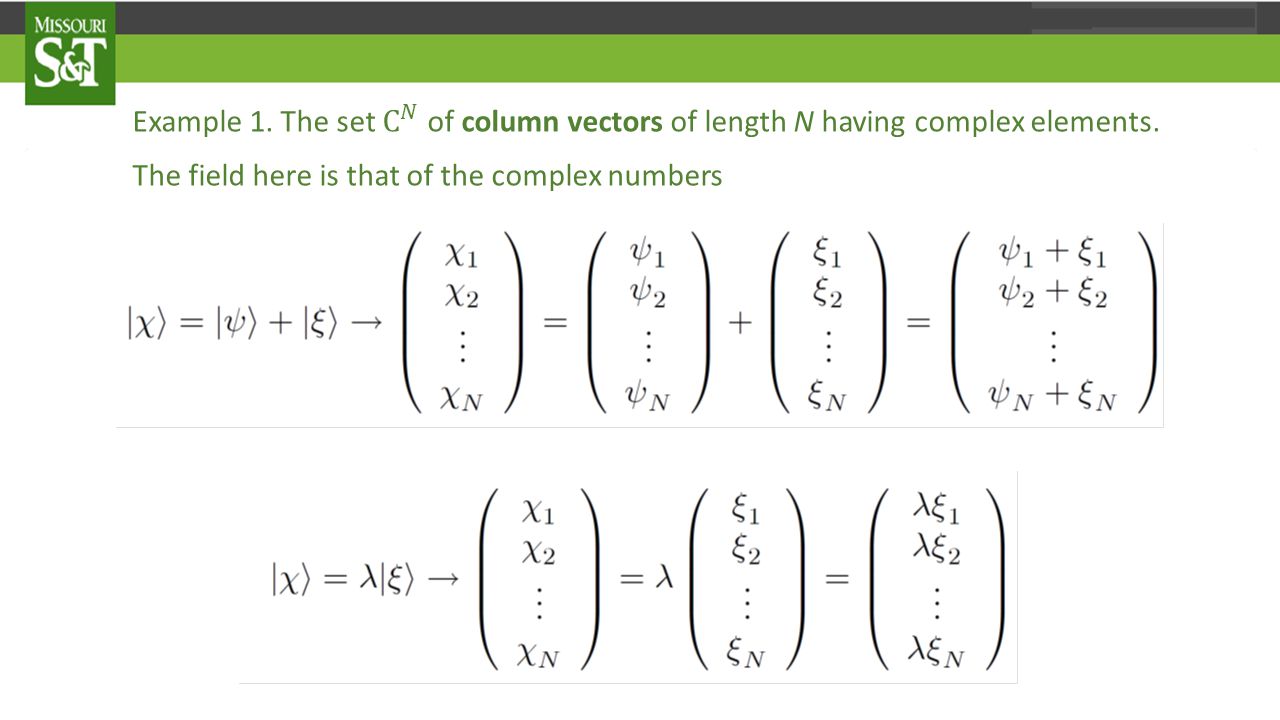
40. The notation (due to Dirac) distinguishes vectors |ξ 〉 of S from scalars λ (elements of the field) and is similar to the use of arrows, boldface symbols, etc. to distinguish vectors in R³ from their scalar counterparts. Let us consider some mathematical examples of vector spaces more relevant to quantum mechanics. Note: In all cases of quantum mechanical interest the relevant field is the set C of complex numbers. In quantum mechanics we are interested in complex vector spaces. (as stated explicitly in the first postulate)

41. The notation (due to Dirac) distinguishes vectors |ξ 〉 of S from scalars λ (elements of the field) and is similar to the use of arrows, boldface symbols, etc. to distinguish vectors in R³ from their scalar counterparts. Let us consider some mathematical examples of vector spaces more relevant to quantum mechanics. Note: In all cases of quantum mechanical interest the relevant field is the set C of complex numbers. In quantum mechanics we are interested in complex vector spaces. (as stated explicitly in the first postulate)

42. The notation (due to Dirac) distinguishes vectors |ξ 〉 of S from scalars λ (elements of the field) is similar to the use of arrows, boldface symbols, etc. to distinguish vectors in R³ from their scalar counterparts. Let us consider some mathematical examples of vector spaces more relevant to quantum mechanics. Note: In all cases of quantum mechanical interest the relevant field is the set C of complex numbers. In quantum mechanics we are interested in complex vector spaces. (as stated explicitly in the first postulate)

46. Example 2. The set L²(Rⁿ) of complex-valued square-integrable functions ψ on Rⁿ. By definition, the function ψ(x) is in L²(R) if the integral exists and is non-infinite. Again the field is that of the complex numbers and vector addition is associated with the pointwise addition and multiplication of functions, i.e.,: |χ 〉 =|ψ 〉 +|ξ 〉 → χ(x)=ψ(x)+ξ(x) |χ 〉 =λ|ξ 〉 → χ(x)=λξ(x) Note that all we are doing here is "adding by components", as in the example above, except that in this circumstance the components are labeled by a continuous index x, instead of a discrete one.

47. Example 2. The set L²(Rⁿ) of complex-valued square-integrable functions ψ on Rⁿ. By definition, the function ψ(x) is in L²(R) if the integral exists and is non-infinite. Again the field is that of the complex numbers and vector addition is associated with the pointwise addition and multiplication of functions, i.e.,: Note that all we are doing here is "adding by components", as in the example above, except that in this circumstance the components are labeled by a continuous index x, instead of a discrete one.

48. Example 2. The set L²(Rⁿ) of complex-valued square-integrable functions ψ on Rⁿ. By definition, the function ψ(x) is in L²(R) if the integral exists and is non-infinite. Again the field is that of the complex numbers and vector addition is associated with the pointwise addition and multiplication of functions, i.e.,: Note that all we are doing here is "adding by components", as in the example above, except that in this circumstance the components are labeled by a continuous index x, instead of a discrete one.

49. Example 2. The set L²(Rⁿ) of complex-valued square-integrable functions ψ on Rⁿ. By definition, the function ψ(x) is in L²(R) if the integral exists and is non-infinite. Again the field is that of the complex numbers and vector addition is associated with the pointwise addition and multiplication of functions, i.e.,: Note that all we are doing here is "adding by components", as in the example above, except that in this circumstance the components are labeled by a continuous index x, instead of a discrete one.

50. Example 2. The set L²(Rⁿ) of complex-valued square-integrable functions ψ on Rⁿ. By definition, the function ψ(x) is in L²(R) if the integral exists and is non-infinite. Again the field is that of the complex numbers and vector addition is associated with the pointwise addition and multiplication of functions, i.e.,: Note that all we are doing here is "adding by components", as in the example above, except that in this circumstance the components are labeled by a continuous index x, instead of a discrete one.

51. Example 2. The set L²(Rⁿ) of complex-valued square-integrable functions ψ on Rⁿ. By definition, the function ψ(x) is in L²(R) if the integral exists and is non-infinite. Again the field is that of the complex numbers and vector addition is associated with the pointwise addition and multiplication of functions, i.e.,: Note that all we are doing here is "adding by components", as in the example above, except that in this circumstance the components are labeled by a continuous index x, instead of a discrete one.

52. The set L²(Rⁿ) of square integrable functions does not include the plane waves (momentum eigenfunctions), or delta functions (position eigenfunctions), so its useful to enlarge the space by considering the set of F(Rⁿ) of Fourier representable functions, i.e., those whose Fourier transform exists. This includes plane waves, whose Fourier transforms are delta functions, and delta functions, whose Fourier transforms are plane waves (work it out and see!) The set L²(Rⁿ) of square integrable functions is actually a subset of the set F(Rⁿ) of Fourier representable functions, and since it is, by itself, a linear vector space under the same operations of vector addition and scalar multiplication defined in F(Rⁿ), it is referred to as a subspace of F(Rⁿ). Definition: A subset S’ ⊂ S, which is, by itself, a linear vector space under the same operations of vector addition and scalar multiplication as defined in S is referred to as a subspace of S.

53. The set L²(Rⁿ) of square integrable functions does not include the plane waves (momentum eigenfunctions), or delta functions (position eigenfunctions), so its useful to enlarge the space by considering the set of F(Rⁿ) of Fourier representable functions, i.e., those whose Fourier transform exists. This includes plane waves, whose Fourier transforms are delta functions, and delta functions, whose Fourier transforms are plane waves (work it out and see!) The set L²(Rⁿ) of square integrable functions is actually a subset of the set F(Rⁿ) of Fourier representable functions, and since it is, by itself, a linear vector space under the same operations of vector addition and scalar multiplication defined in F(Rⁿ), it is referred to as a subspace of F(Rⁿ). Definition: A subset S’ ⊂ S, which is, by itself, a linear vector space under the same operations of vector addition and scalar multiplication as defined in S is referred to as a subspace of S.

54. The set L²(Rⁿ) of square integrable functions does not include the plane waves (momentum eigenfunctions), or delta functions (position eigenfunctions), so its useful to enlarge the space by considering the set of F(Rⁿ) of Fourier representable functions, i.e., those whose Fourier transform exists. This includes plane waves, whose Fourier transforms are delta functions, and delta functions, whose Fourier transforms are plane waves (work it out and see!) The set L²(Rⁿ) of square integrable functions is actually a subset of the set F(Rⁿ) of Fourier representable functions, and since it is, by itself, a linear vector space under the same operations of vector addition and scalar multiplication defined in F(Rⁿ), it is referred to as a subspace of F(Rⁿ). Definition: A subset S’ ⊂ S, which is, by itself, a linear vector space under the same operations of vector addition and scalar multiplication as defined in S is referred to as a subspace of S.

55. The set L²(Rⁿ) of square integrable functions does not include the plane waves (momentum eigenfunctions), or delta functions (position eigenfunctions), so its useful to enlarge the space by considering the set of F(Rⁿ) of Fourier representable functions, i.e., those whose Fourier transform exists. This includes plane waves, whose Fourier transforms are delta functions, and delta functions, whose Fourier transforms are plane waves (work it out and see!) The set L²(Rⁿ) of square integrable functions is actually a subset of the set F(Rⁿ) of Fourier representable functions, and since it is, by itself, a linear vector space under the same operations of vector addition and scalar multiplication defined in F(Rⁿ), it is referred to as a subspace of F(Rⁿ). Definition: A subset S’ ⊂ S, which is, by itself, a linear vector space under the same operations of vector addition and scalar multiplication as defined in S is referred to as a subspace of S.

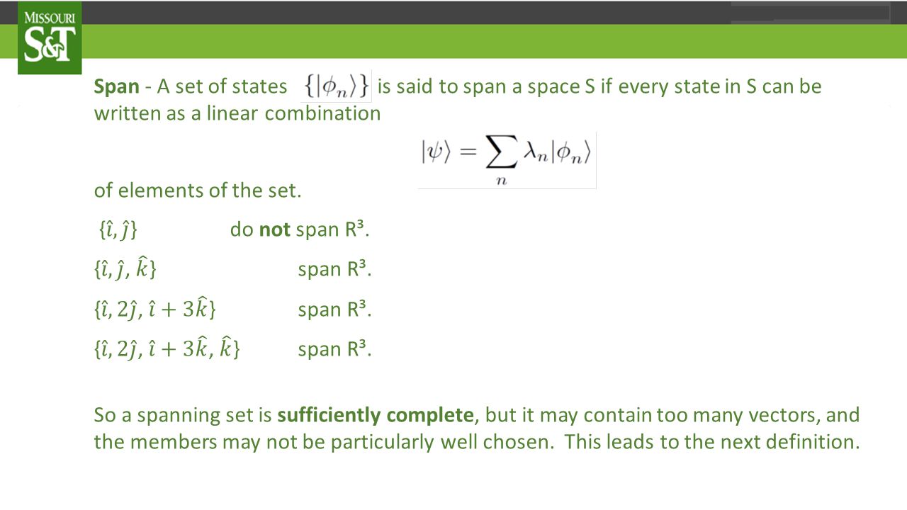
56. This idea of a subspace will be very important to us. Geometrically, it is not hard to see that the set of position vectors lying in the xy- plane forms a 2-dimensional subspace of the set of all position vectors in R³. The set of all vectors lying along the z axis forms a 1-dimensional subspace of R³. To proceed we need to provide some additional definitions. We first introduce the notion of a spanning set of vectors:

57. This idea of a subspace will be very important to us. Geometrically, it is not hard to see that the set of position vectors lying in the xy- plane forms a 2-dimensional subspace of the set of all position vectors in R³. The set of all vectors lying along the z axis forms a 1-dimensional subspace of R³. To proceed we need to provide some additional definitions. We first introduce the notion of a spanning set of vectors:

58. This idea of a subspace will be very important to us. Geometrically, it is not hard to see that the set of position vectors lying in the xy- plane forms a 2-dimensional subspace of the set of all position vectors in R³. The set of all vectors lying along the z axis forms a 1-dimensional subspace of R³. To proceed we need to provide some additional definitions. We first introduce the notion of a spanning set of vectors:

59. This idea of a subspace will be very important to us. Geometrically, it is not hard to see that the set of position vectors lying in the xy- plane forms a 2-dimensional subspace of the set of all position vectors in R³. The set of all vectors lying along the z axis forms a 1-dimensional subspace of R³. To proceed we need to provide some additional definitions. We first introduce the notion of a spanning set of vectors:

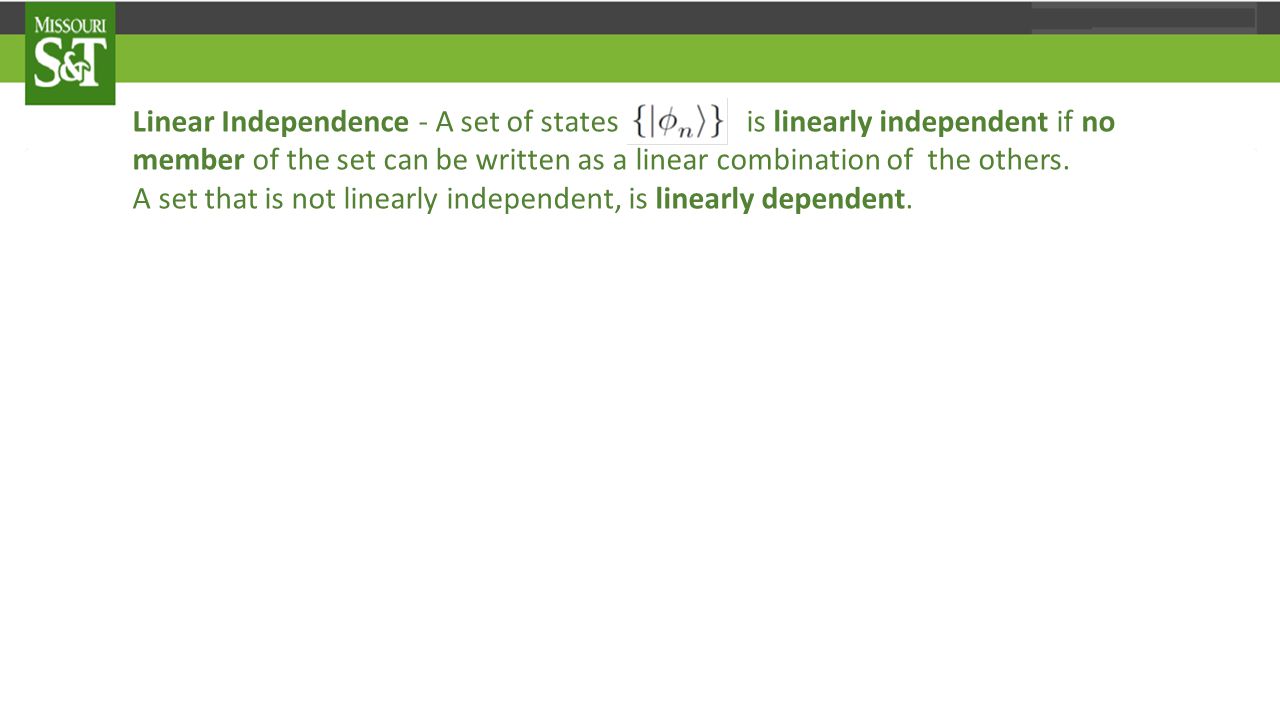
73. Dimension - If a linear vector space S contains a subset of N linearly independent vectors, but does not contain a subset of N+1 linearly independent vectors it has dimension N, or is an N-dimensional space. If there exist subsets of S with N linearly independent vectors for all N, it is said to be infinite dimensional. Many quantum state spaces are of infinite dimension. R³ is a three dimensional vector space. Basis - A linearly independent set of states that spans S forms a basis for the space. A basis set is often referred to as being complete with respect to the vector space that it spans, i.e., it forms a complete set of states for the space.

74. Dimension - If a linear vector space S contains a subset of N linearly independent vectors, but does not contain a subset of N+1 linearly independent vectors it has dimension N, or is an N-dimensional space. If there exist subsets of S with N linearly independent vectors for all N, it is said to be infinite dimensional. Many quantum state spaces are of infinite dimension. R³ is a three dimensional vector space. Basis - A linearly independent set of states that spans S forms a basis for the space. A basis set is often referred to as being complete with respect to the vector space that it spans, i.e., it forms a complete set of states for the space.

75. Dimension - If a linear vector space S contains a subset of N linearly independent vectors, but does not contain a subset of N+1 linearly independent vectors it has dimension N, or is an N-dimensional space. If there exist subsets of S with N linearly independent vectors for all N, it is said to be infinite dimensional. Many quantum state spaces are of infinite dimension. R³ is a three dimensional vector space. Basis - A linearly independent set of states that spans S forms a basis for the space. A basis set is often referred to as being complete with respect to the vector space that it spans, i.e., it forms a complete set of states for the space.

76. Dimension - If a linear vector space S contains a subset of N linearly independent vectors, but does not contain a subset of N+1 linearly independent vectors it has dimension N, or is an N-dimensional space. If there exist subsets of S with N linearly independent vectors for all N, it is said to be infinite dimensional. Many quantum state spaces are of infinite dimension. R³ is a three dimensional vector space. Basis - A linearly independent set of states that spans S forms a basis for the space. A basis set is often referred to as being complete with respect to the vector space that it spans, i.e., it forms a complete set of states for the space.

77. Dimension - If a linear vector space S contains a subset of N linearly independent vectors, but does not contain a subset of N+1 linearly independent vectors it has dimension N, or is an N-dimensional space. If there exist subsets of S with N linearly independent vectors for all N, it is said to be infinite dimensional. Many quantum state spaces are of infinite dimension. R³ is a three dimensional vector space. Basis - A linearly independent set of states that spans S forms a basis for the space. A basis set is often referred to as being complete with respect to the vector space that it spans, i.e., it forms a complete set of states for the space.

78. Note that by definition, any spanning set of vectors contains a basis as a subset. (We just have to weed out any unnecessary vectors which can themselves be written as linear combinations of the remaining ones.) Perhaps the most useful distinction between a basis set and a spanning set, is that the expansion coefficients expressing any element of the space in terms of the members of a basis are unique. That is, if form a basis for S, and |ψ 〉 is an arbitrary element of S it can be written as a linear combination in terms of these vectors in only one way. This is easy to prove. Assume that there existed another expansion but then so

79. Note that by definition, any spanning set of vectors contains a basis as a subset. (We just have to weed out any unnecessary vectors which can themselves be written as linear combinations of the remaining ones.) Perhaps the most useful distinction between a basis set and a spanning set, is that the expansion coefficients expressing any element of the space in terms of the members of a basis are unique. That is, if form a basis for S, and |ψ 〉 is an arbitrary element of S it can be written as a linear combination in terms of these vectors in only one way. This is easy to prove. Assume that there existed another expansion but then so

80. Note that by definition, any spanning set of vectors contains a basis as a subset. (We just have to weed out any unnecessary vectors which can themselves be written as linear combinations of the remaining ones.) Perhaps the most useful distinction between a basis set and a spanning set, is that the expansion coefficients expressing any element of the space in terms of the members of a basis are unique. That is, if form a basis for S, and |ψ 〉 is an arbitrary element of S it can be written as a linear combination in terms of these vectors in only one way. This is easy to prove. Assume that there existed another expansion but then so

81. Note that by definition, any spanning set of vectors contains a basis as a subset. (We just have to weed out any unnecessary vectors which can themselves be written as linear combinations of the remaining ones.) Perhaps the most useful distinction between a basis set and a spanning set, is that the expansion coefficients expressing any element of the space in terms of the members of a basis are unique. That is, if form a basis for S, and |ψ 〉 is an arbitrary element of S it can be written as a linear combination in terms of these vectors in only one way. This is easy to prove. Assume that there existed another expansion but then so

82. Note that by definition, any spanning set of vectors contains a basis as a subset. (We just have to weed out any unnecessary vectors which can themselves be written as linear combinations of the remaining ones.) Perhaps the most useful distinction between a basis set and a spanning set, is that the expansion coefficients expressing any element of the space in terms of the members of a basis are unique. That is, if form a basis for S, and |ψ 〉 is an arbitrary element of S it can be written as a linear combination in terms of these vectors in only one way. This is easy to prove. Assume that there existed another expansion but then so

83. Note that by definition, any spanning set of vectors contains a basis as a subset. (We just have to weed out any unnecessary vectors which can themselves be written as linear combinations of the remaining ones.) Perhaps the most useful distinction between a basis set and a spanning set, is that the expansion coefficients expressing any element of the space in terms of the members of a basis are unique. That is, if form a basis for S, and |ψ 〉 is an arbitrary element of S it can be written as a linear combination in terms of these vectors in only one way. This is easy to prove. Assume that there existed another expansion but then so

84. Note that by definition, any spanning set of vectors contains a basis as a subset. (We just have to weed out any unnecessary vectors which can themselves be written as linear combinations of the remaining ones.) Perhaps the most useful distinction between a basis set and a spanning set, is that the expansion coefficients expressing any element of the space in terms of the members of a basis are unique. That is, if form a basis for S, and |ψ 〉 is an arbitrary element of S it can be written as a linear combination in terms of these vectors in only one way. This is easy to prove. Assume that there existed another expansion but then so

85. As a final definition before we close this lecture, its useful to define a form of the word span that is a noun, rather than a verb. Given any set of vectors, we can consider the set S′ = { } of all possible linear combinations of members of the set. This a set is closed under vector addition and scalar multiplication, and thus forms a subspace of S. We will refer to this subspace S′ as the span of, and denote it by S′=Span( ). Clearly, if the set of vectors is complete, then its span is the entire space S itself.

86. So in this lecture, we stated the first postulate of the general form of quantum mechanics, and we worked our way through a lot of definitions that will be absolutely crucial if we want to understand the mathematical structure of quantum mechanics. In giving these definitions we considered sets of vectors labeled by a discrete index. But we will often encounter sets of states that are labeled by a continuous index. In the next lecture, we extend our definitions to include sets of this type, and work our way towards general notions of length and direction in our quantum mechanical state space, by introducing the idea of an inner product.

87. So in this lecture, we stated the first postulate of the general form of quantum mechanics, and we worked our way through a lot of definitions that will be absolutely crucial if we want to understand the mathematical structure of quantum mechanics. In giving these definitions we considered sets of vectors labeled by a discrete index. But we will often encounter sets of states that are labeled by a continuous index. In the next lecture, we extend our definitions to include sets of this type, and work our way towards general notions of length and direction in our quantum mechanical state space, by introducing the idea of an inner product.

88. So in this lecture, we stated the first postulate of the general form of quantum mechanics, and we worked our way through a lot of definitions that will be absolutely crucial if we want to understand the mathematical structure of quantum mechanics. In giving these definitions we considered sets of vectors labeled by a discrete index. But we will often encounter sets of states that are labeled by a continuous index. In the next lecture, we extend our definitions to include sets of this type, and work our way towards general notions of length and direction in our quantum mechanical state space, by introducing the idea of an inner product.

89. So in this lecture, we stated the first postulate of the general form of quantum mechanics, and we worked our way through a lot of definitions that will be absolutely crucial if we want to understand the mathematical structure of quantum mechanics. In giving these definitions we considered sets of vectors labeled by a discrete index. But we will often encounter sets of states that are labeled by a continuous index. In the next lecture, we extend our definitions to include sets of this type, and work our way towards general notions of length and direction in our quantum mechanical state space, by introducing the idea of an inner product.