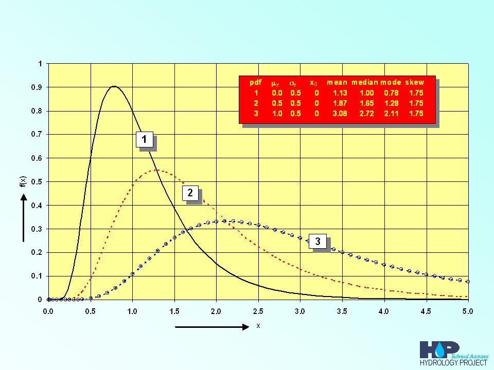
1. Parameters of distribution
Location Parameter
Scale Parameter
Shape Parameter

5. Plotting position
Plotting position of xi means, the probability assigned to each data point to be plotted on probability paper.
The plotting of ordered data on extreme probability paper is done according to a general plotting position function:
P = (m-a) / (N+1-2a).
Constant 'a' is an input variable and is default set to 0.3.
Many different plotting functions are used, some of them can be reproduced by changing the constant 'a'.
Gringorton P = (m-0.44)/(N+0.12) a = 0.44
Weibull P = m/(N+1) a = 0
Chegadayev P = (m-0.3)/(N+0.4) a = 0.3
Blom P = (m-0.375)/(N+0.25) a = 0.375

6. Curve Fitting Methods
The method is based on the assumption that the observed data follow the theoretical distribution to be fitted and will exhibit a straight line on probability paper.
Graphical Curve fitting Method
Mathematical Curve fitting Method.-
Method of Moments-
Method of Least squares
Method of Maximum Likelihood

7. Estimation of statistical parameters
To apply theoretical distribution functions following steps are required:
investigate homogeneity of series
estimate the parameters of postulated distribution
test goodness of fit of theoretical distribution to observed frequency distribution
Estimation of parameters:
graphical method
analytical methods:
method of moments
maximum likelihood method
method of least squares
mixed moment-maximum likelihood method

8. Estimation of statistical parameters (2)
Estimation procedures differ
Comparison of quality by:
mean square error or its root
error variance and standard error
bias
efficiency
consistency
Mean square error in  of :

9. Estimation of statistical parameters (3)
Consequently:
First part is the variance of  = average of squared differences about expected mean, it gives the random portion of the error
Second part is square of bias, bias = systematic difference between expected and true mean, it gives the systematic portion of the error
Root mean square error:
Standard error
Consistency:
Mind effective number of data

10. Graphical estimation Variable is function of reduced variate:
e.g. for Gumbel:
Reduced variate function of non-exceedance prob.:
Determine non-exceedance prob. from rank number of data in ordered set, e.g. for Gumbel:
Unbiased plotting position depends on distribution

11. Graphical estimation (2)
Procedure:
rank observations in ascending order
compute non-exceedance frequency Fi
transform Fi into reduced variate zi
plot xi versus zi
draw straight line through points by eye-fitting
estimate slope of line and intercept at z = 0 to find the parameters

12. Graphical estimation: example
Annual maximum river flow at Chooz on Meuse

13. Graphical estimation

14. Graphical estimation: example (2)
Gumbel parameters:
graphical estimation: x0 = 590,  = 247
MLM-method: x0 = 591,  = 238
100-year flood:
T = 100  FX(x) = 1-1/100 = 0.99
z = -ln(-ln(0.99)) = 4.6
graphical method: x = x0 + z = x4.6 = 1726 m3/s
MLM method: x = x0 + z = x4.6 = 1686 m3/s
Graphical method: pro’s and con’s
easily made
visual inspection of series
strong subjective element in method: not preferred for design; only useful for first rough estimate
confidence limits will be lacking

15. Plotting positions Plotting positions should be: General: unbiased
minimum variance
General:

16. Product moment Standard procedure: In HYMOS method available for:
estimate mean and variance for 2-par distributions
estimate mean, variance and skewness for 3-par distr.
In HYMOS method available for:
normal
LN-2 & LN-3
G-2 & P-3
EV-1
Pro’s and con’s of Method:
simple procedure
for small sample sizes ( N < 30) sample moments may substantially differ from population values, due to too much weight to outliers
3-parameters from small samples provides poor quality estimates

17. PWM and L-moments Definition of Probability weighted moments (PWM):
Choose p=1 and s=0:
It follows that in PWM the non-exceedance probability is raised to a power, rather than the variable itself
Since FX(x) < 1 PWM’s are much less sensitive for outliers
But: higher weight is put on higher ranked values

18. L-moments Order statistics (data in ascending order):
then Xi:N is ith order statistic
first four L-moments:

19. L-moments (2) L-skewness and L-kurtosis:
Relation of L-moments with distribution parameters:
Normal Gumbel

20. L-moments and PWM
Determination of L-moments requires numerous combination = cumbersome
Relation between L-moments and PWM:

21. Sample estimates of PWM’s

22. Example L-moments
Higher weight on higher ranked values

23. Example L-moments (2)

24. L-moment diagram

25. Maximum likelihood method
Principle:
Given r.v. X with pdf fX(x) and sample of X of size N
pdf fX(x) has parameters 1, 2,…,k
sample values independent and identically distributed
then with parameter set  the prob. that r.v. will fall in interval including xi is given by: pdf fX(xi|)dx
joint prob. of occurrence of sample set xi, i=1 to N is
procedure involves maximisation of:

26. Maximum likelihood method (2)
Likelihood function:
Best set of parameters follow from:
Log-likelihood maximisation often easier, since products are replaced by sums:

27. Example MLM LN-2 distribution: Likelihood for sample of N is:
Log-likelihood:
Parameters follow from:

28. Example MLM Parameters for LN-2:
Parameters are seen to be first and second moments about origin and mean of ln(x)
Similarly the parameters for LN-3 can be derived
Equations become more complicated
For small samples convergence is poor
then mixed-moment MLM method is preferred

29. Parameter estimation by Least Squares
Method is extension of graphical method
Instead of fitting line by eye, the Least Squares method is used
Quality of method strongly dependent on probability assigned to ranked sample values (plotting position)
Example of annual flow extremes of Meuse at Chooz carried out using Gringorten and Weibull plotting position
Difference for 100 year flood is resp. 3% and 9% with MLM estimate
Weibull plotting position gives low T to highest sample value, hence in extrapolated part higher values are found than e.g. with Gringorten

30. Method of Least Squares

31. Mixed-moment maximum likelihood method
Method applies generally MLM to 2 parameters and the product moment method to the location parameter
Example is for LN-3:
use MLM-estimates with X replaced by X - x0:
The location parameter is taken from the first moment:

32. Mixed-moment max.likelihood meth. (2)
The location parameter is solved iteratively
the following modified form is used:
For each value of x0 : Y and Y2 are estimated using Newton-Raphson method:
the denominator is estimated by its expected value:
The new x0 is determined (until improvement is small) from:

33. Censoring of data
Right censoring: eliminating data from analysis at the high side of the data set
Left censoring: eliminating data from analysis at the low side of the data set
Relative frequencies of remaining data is left unchanged.
Right censoring may be required because:
extremes in data set have higher T than follows from series
extremes may not be very accurate
Left censoring may be required because:
physics of lower part is not representative for higher values

35. Quantile uncertainty and confidence limits
Estimation errors in parameters lead to estimation errors in quantiles
Procedure demonstrated for quantile of N(X, X2)
quantile estimated by:
estimation variance of quantile:
Hence:
Var mX = sX2/N
Var (sX) = sX2/2N
Cov(mX,sX) =0

36. Quantile uncertainty and conf. limits (2)
Confidence limits become:
CL diverge away from the mean
Number of data N also determine width of CL
Uncertainty in non-exceedance probability for a fixed xp:
standard error of reduced variate
It follows with zp approx N(zp,zp):
hence:

37. Confidence limits for frequency distribution

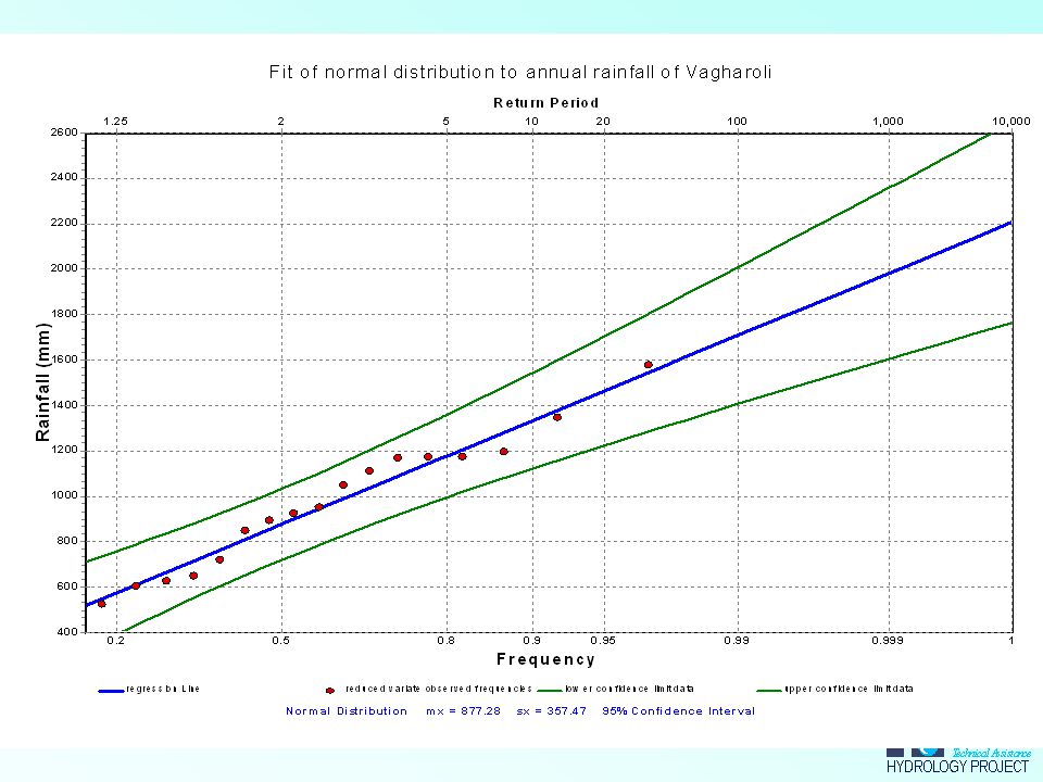
38. Example rainfall Vagharoli

39. Example rainfall Vagharoli (2)
Normal distribution
FX(z) for
z=(x-877)/357
Ranked observations
T=1/(1-FX(z))
Fi=(i-3/8)/(N+1/4)

40. Example rainfall Vagharoli (3)

41. Example Vagharoli (4) T
FX(x) = 1 - 1/T

43. Investigating homogeneity
Prior to fitting, tests required on:
1. stationarity (properties do not vary with time)
2. homogeneity (all element are from the same population)
3. randomness (all series elements are independent)
First two conditions transparent and obvious. Violating last condition means that effective number of data reduces when data are correlated
lack of randomness may have several causes; in case of a trend there will be serial correlation
HYMOS includes numerous statistical test :
parametric (sample taken from appr. Normal distribution)
non-parametric or distribution free tests (no conditions on distribution, which may negatively affect power of test

44. Summary of tests On randomness: On correlation: On homogeneity:
median run test
turning point test
difference sign test
On correlation:
Spearman rank correlation test
Spearman rank trend test
Arithmetic serial correlation coefficient
Linear trend test
On homogeneity:
Wilcoxon-Mann-Whitney U-test
Student t-test
Wilcoxon W-test
Rescaled adjusted range test

45. Chi-square goodness of fit test
Hypothesis
F(x) is the distribution function of a population from which sample xi, i =1,…,N is taken
Actual to theoretical number of occurrences within given classes is compared
Procedure:
data set is divided in k class intervals containing at least each 5 values
Class limits from all classes have equal probability
pj = 1/k = F(zj) - F(zj-1)
e.g. for 5 classes this is p = 0.20, 0.40, 0.60, 0.80 and 1.00
the interval j contains all xi with: UC(j-1)<xi UC(j)
the number of samples falling in class j = bj is computed
the number of values expected in class j = ej according to the theoretical distribution is computed
the theoretical number of values in any class = N/k because of the equal probability in each class

46. Chi-squared goodness of fit test

47. Chi-square goodness of fit test (2)
Consider following test statistic:
under H0 test statistic has 2 distr, with df  = k-1-m
k= number classes, m = number of parameters
simplified test statistic:
H0 not rejected at significance level  if:

48. Number of classes in Chi-squared goodness of fit test

49. Example Annual rainfall Vagharoli (see parameter estimation)
test on applicability of normal distribution
4 class intervals were assumed (20 data)
upper class levels are at p=0.25, 0.50, 0.75 and 1.00
the reduced variates are at , 0.00, and 
hence with mean = 877, and stdv = 357 the class limits become: x357 = 636
= 877
x357 = 1118 

50. Example continued (2)
From the table it follows for the test statistic:
At significance level  = 5%, according to Chi-squared distribution for  = df the critical value is at 3.84, hence c2 < critical value, so H0 is not rejected