1. starting from 300MHZ to about 60GHZ
This is Microwave
starting from 300MHZ to about 60GHZ
CHAPTER 0

2. a) Basic notions in Radio Propagation at microwave frequencies,
  The aim of this Course is to Give
a) Basic notions in Radio Propagation at microwave frequencies,
b) application to Radio Link Design in the frequency range from about 450 MHz up to 60 GHz.
Means :
- Course notes
- Lab simulators

3. - Modulation techniques, - Radio equipment and systems
  Prerequisites: - basic notions in:
- Modulation techniques,
- Radio equipment and systems
- Elementary electromagnetic physics.
Conclusion :
Course objective : actively involving the reader in navigating through the text and in practicing with exercises in the field of microwave link design. 

4. Introduction To MW links
In telecommunications, information can be analog or digital.
since the 1970’s , MW Analog systems have been almost completely replaced by digital systems.
Now even analog traffic, such as voice calls, are converted to digital signals ( sampling), to facilitate long distance transmission and switching.

5. Terrestrial MW systems have been used since the 1950’s( wartime radar technology).
Today, modern digital microwave radio is world widely deployed to transport information over distances of up to 60 kilometers ( sometimes farther).
Microwave radio is totally transparent to the information carried : which can be voice, data, video, or a combination of all three.

6. Transport can be in a variety of formats :
circuit-switched Time Division Multiplex
(TDM)
packet-based data protocols such as ATM,
Frame Relay or IP, Ethernet.
In some cases, packetized data can be overlaid on a TDM frame structure such as:
- PDH,
- SDH or SONET.

7. Microwave radio advantages over cable/fiber-based transmission:
Rapid Deployment
No right-of-way issues – avoid all obstacles
Any requirement to seek permissions :cost & time delays.
Flexibility: simple redeployment & capacity adjustment.

8. Operator-owned infrastructure - no reliance on competitors.
Losing customers ≠ Losing assets as in Cables & fibers
Easily crosses city terrain (extremely restricted,& very expensive, to install fiber in city terrains and street crosses).
Operator-owned infrastructure - no reliance on competitors.
Low start-up capital costs : independent of the link distance.

9. Minimal operational costs.
Radio infrastructure already exists (rooftops, masts and towers).
Microwave radio is not susceptible to catastrophic failure ( cable cuts,) and can be repaired in minutes instead of hours or days.
Better resistance to natural disasters (flood, earthquakes).
where the fiber was not always available (the radio is only choice)

10. Fiber is very cost effective where extremely high bandwidths are required.
However, in the access portion of the network, where the maximum capacity requirements are less than STM-4, radio has an obvious advantage.
Note STM1 = 155 Mbits ; STMn = n*155Mbits

11. The 3 basic components of the radio terminal
Two radio terminals are required to establish a MW “hop”.
1- digital modem interfaces with digital terminal equipment, converting customer traffic to a modulated radio signal;
2- a radio frequency (RF) unit : Frequency converter + RF amplifier up to around 1 watt.
3- a passive parabolic antenna to transmit and receive the signal.

12. 2-Basic configurations for MW terminals
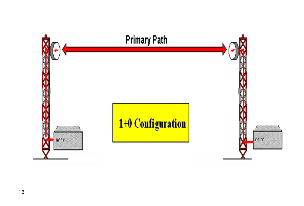
1-Non-protected, ( 1+0) :
- Any major failure component will result in
a loss of customer traffic.
- cost-effective when traffic is non-critical, or where
alternate traffic routing is available.
2-protected (1+1) : Main + hot standby (Monitored Hot Standby (MHSB))
- twice expensive, but No loss of customer traffic.

15. 3- Space Diversity
4- Frequency Diversity
5- Polarization diversity
6-Angle diversity
In addition, Some radios are fitted to use ODU attached directly to the back of the antenna, eliminating antenna feed lines and attendant feed line losses).

16. Used to reinforce the radio dispersive fade margin
Used to reinforce the radio dispersive fade margin . The new technology of Mw radio don’t need this type of diversity

18. Two very important characteristic of digital MW transmission is:
A- immunity to noise
B- the ability of the radio to operate in the presence of adverse environmental conditions.

19. A- immunity to noise
Noise refers to the effects caused by unwanted electromagnetic signals that interfere and corrupt the received signal.

20. Microwave systems operate in so-called “licensed” frequency bands between 2 and 38 GHz (tightly regulation the use of these frequencies ensure that each operator will not cause interference to other links operating in the same area).
The frequency band characteristics are also tightly specified on a worldwide basis by ITU.

21. Equipment are controlled, to meet stringent specifications ( ITU standards, National as FCC and ETSI).
This is in contrast to the “unlicensed” frequency bands of 2.4 and 5.8 GHz :
No control, Unlicensed systems themselves incorporate countermeasures to avoid noise and interference, such as spread-spectrum transmission

22. B- the ability of the radio to operate in the presence of adverse environmental conditions.
a perception that microwave is still unreliable due to “fading” .
This is largely a remnant of the analog days.
However, digital radio systems today are able to counteract fading effects in a number of ways

23. Fading is known to occur as a result of primarily two phenomena.
1- Firstly, multipath interference affects mainly lower frequencies below 18 GHz.
This happens when the reflected signal arrive slightly later than the direct signal path .it reduces the ability of the receiver to correctly distinguish the data carried on the signal.

24. Fortunately, modern radio systems can compensate for this form of interference through countermeasures such as:
signal equalization [using DSP-filtering to cancel the echoes (pre-echoes & post-echoes) due to Multipath].
Forward Error Correction,
diversity receiver configurations.
Multipath fade measurement parameter is often called the reliability of the link ) ( (ذا ثقة)-

25. 2-
Secondly, precipitation, mostly in the form of rain, can severely affect microwave radio systems in the higher frequencies above 18 GHz.
Microwaves cannot penetrate rain, so :
the heavier the downpour, and the higher the frequency, the greater the signal attenuation.
Rain fade measurement parameter is often called the availability of the link

26. Although there is noway to counteract rain fade other than higher transmission power.
The mechanisms of rain fade are very well understood:
models have been developed by the ITU to enable links to be planned within extremely accurate tolerances based upon particular rainfall profiles.

27. Conclusion :
As a result, modern microwave systems can be designed for extremely high link total availabilities in excess of %, translating to link downtimes of literally seconds annually, which is easily comparable to that provided by supposed “error-free” optical fiber systems.
Note : total availability concerns the 2 types of the fade

28. Microwave applications
Mobile Cellular Networks
to provide service for customers and to generate immediate revenue, cellular carriers need to connect their cell sites to switching stations, and have chosen microwave due to:
its reliability
speed of deployment
cost benefits over fiber or leased-line alternatives.

29. Microwave radio will be heavily deployed in the emerging 2
Microwave radio will be heavily deployed in the emerging 2.5 and 3G mobile infrastructures: More data usage
greater numbers of cell sites.

30. Last Mile Access
A significant proportion of business premises lack broadband connectivity : Wireless provides the perfect medium for connecting new customers to overcome the last mile bottleneck.
Even if an operator chooses to use unlicensed or multi-point wireless technologies to connect customers, high capacity microwave provides the ideal solution for backhaul of customer traffic from access hubs to the nearest fiber

31. Private Networks:
Companies now have high speed LAN / WAN network requirements and need to connect parts of their business in the same campus, city or country.
Microwave radio is able to provide rapid, high capacity connections that are compatible with Fast and Gigabit Ethernet data networks, enabling LANs to be extended without reliance on fiber build-out.

32. Disaster Recovery
Natural (earthquakes, floods, hurricanes ) and man-made (terrorist attack and wars) disasters can wreak havoc on a communications network:
Microwave is often used to restore communications when transmission equipment has been damaged by or other natural disasters, or man-made conflicts such as ( Kuwait, Serbia and Kosovo)

33. The Digital Divide
Microwave radio plays a key role in bridging the digital divide :
quickly establish a network of access hubs and high-speed backhaul network to bring advanced communications services to areas that would normally have to wait.

34. Developing Nations
Microwave has traditionally allowed developing nations the means of establishing state-of-the-art telecommunications quickly over often undeveloped and impractical terrain ( deserts, jungle or frozen terrain where laying cable would be all but impossible.

35. Control and Monitoring
Public transport organizations, railroads, and other public utilities are major users of microwave.
These companies use microwave to carry control and monitoring information to and from power substations, pumping stations, and switching stations.

36. Chapter 1
This is the DB

37. CH 1- what are the decibels
A- Understanding db & db units :
A- db : The ratio of 2 signals may be expressed in db by :
in case of voltages : V1/V2
( V2/V1)db = 20 log10 ( V2/V1)
in case of Powers : P1/P2
( P2/P1)db = 10 log10 ( P2/P1)

38. Example :
a signal if 10 w is applied to long transmission line . The power measured at the load end is 7 W. What is the loss in db
Solution :

39. Table of some common ratios
Voltage ratio (db)
20 log10 R
Power ratio (db)
10 log10 R
Factor
Ratio ®
0.00 1
1:1 6
3.01 2
2:1 20
10.00 10
10:1 40
20.00
100
100:1 60
30.00
1000
1000:1
-20
-10
0.1
1/10
-40
0.01
1/100
-60
-30
0.001
1/1000

40. 30 dB
is an increase of 1000X in power
20 dB
is an increase of 100X in power
10 dB
is an increase of 10X in power
6 dB
is an increase of 4X in power
3 dB
is an increase of 2X in power
2 dB
is an increase of 1.6X in power
1 dB
is an increase of 1.25X in power
0 dB
is no increase or decrease in power
-1 dB
is a decrease of 20% in power
-2 dB
is a decrease of 37% in power
(roughly a decrease of 1/3)
-3 dB
is a decrease of 50% in power
-6 dB
is a decrease of 75% in power
-10 dB
is a decrease of 90% in power
-20 dB
is a decrease of 99% in power
-30 dB
is a decrease of 99.9% in power

41. B) : - db-power units
- dbw : is the unit of power expressed relatively to 1W
P(dbw) = 10 log10 P(w)
- dbm : is the unit of power expressed relatively to 1mW
P(dbm) = 10 log10 P(mw)
Attention :
0dbw = 30dbm= 1W
0 dbm = -30dbw = 1mw

42. P (dbm) = P(dbW) + 30
P(dbW) = P (dbm) -30

43. Example Problem
If the two antennas in the drawing are "welded" together, how much power in dbm will be measured at point A? (Line loss L1 = L2 = 0.5) –suppose no ideal antenna coupling
Multiple choice: a. 16 dBm b. 28 dBm c. 4 dBm d. 10 dBm e. < 4 dBm

44. Answer:
The antennas do not act as they normally would since the antennas are operating in the near field. They act as inefficient coupling devices resulting in some loss of signal. In addition, since there are no active components, you cannot end up with more power than you started with. The correct answer is "e. < 4 dBm."
10 dBm - 3 dB - small loss -3 dB = 4 dBm - small loss

45. Convert 10dbm in dbw ; -2dbw in dbm
Example :
Convert 10dbm in dbw ; -2dbw in dbm
Solution : given P(dbW) = P (dbm) -30 = = -20 dbW
P (dbm) = P(dbW) + 30 = = 28 dbm
Example : consider the 2 following configurations
10dbm ?
Gain 3db
Gain 10db

46. C) - db-voltage units
- dbmv : is used in RF receiver in which the system
impedance is 50 Ω.
It is the unit of voltage expressed relatively to 1mv
v(dbmv) = 20 log10 v(mv)

47. dbµv : is used in RF receiver in which the system impedance is 50 Ω
dbµv : is used in RF receiver in which the system impedance is 50 Ω. It is the unit of voltage expressed relatively to 1µv :
v(dbµv) = 20 log10 v(µv)
Example : The received RF effective voltage at the input of radio receiver is 0.5mv
. Find the input voltage in dbµv & the input power in dbm
Solution

48. -Field db units : Electromagnetic field
a- Electric field E in dbµv /m
E (dbµv/m) = 20 log10 E (µv/ m)
b- Magnetic field H = E/377 where H in A/m and E in v/ m

50. Power and Field Db-units

51. c) received power in dBm at the RX-antenna
where Gr is the RX-antenna gain.
Pdbm = Edbµv/m + Gr - 20 log (FMHZ) – 77.2
In case of isotropic Rx-antenna
Pdbm = Edbµv/m log (FMHZ) – 77.2
Received voltage into 50 input receiver:
P (dBm) = U (dBµV) - 107

52. Example:
The received RF effective voltage at the input of radio receiver is 0.5mv
a) Find the input voltage in dbµv & the input
power in dbm.
b) knowing that the receiver’s antenna has 20db Gain and the transmitted frequency is 10GHZ,
Find the Electric field at the antenna location In dbµv/m and V/m .
Deduce the Magnetic field value.

53. QUIZ

54. Exercises on Db 
A cable has 6 dB signal loss . Find the signal at the output of this cable ,knowing that the input signal is 1mW.
an amplifier has 15 dB of gain. Find the signal at the output of this amplifier ,knowing that the input signal is 1mW.
Complete the following sentences:
a)Every time you double (or halve) the power level, you add (or subtract) ……. dB to the power level. This corresponds to a ……. percent gain or reduction.
b) ……dB gain/loss corresponds to a tenfold increase/decrease in signal level.
A 20 dB gain/loss corresponds to a ……….-fold
increase/decrease in signal level.

55. Exercises on Dbm (dB milliWatt) A signal strength or power level 0 dBm is defined as …. mW (milliWatt) of power into a terminating load such as an antenna or power meter.
Small signals are negative numbers. For example, typical b WLAN cards have +15 dBm (….mW) of output power. They also specify a -83 dBm (………pW.) RX sensitivity (minimum RX signal level required for 11Mbps reception). Additionally, a) 125 mW is ….. dBm, and
b) ….mW is 24 dBm.

56. Recommended Software Andrew
CH2- Antenna and space
propagation
Recommended Software Andrew

57. Antenna Basic questions
which cause some antennas to accept one wave and reject others?:
The physical size of an antenna : defines the efficiently radiated or received frequency
The shape of the antenna determine the directivity of an antenna
The property of polarization describes the angular pointing of the EM field vector

58. Antenna Electromagnetic field radiation :
General discussion
An antenna serves two basic functions:
1- it matches the characteristic impedance of the transmission line to the intrinsic impedance of free space (To avoid any reflections back to the source or load)
2 - Second, the antenna is designed to direct the electromagnetic radiation in the desired direction.

59. Isotropic Point Radiator
It is a fictitious ideal isotropic point radiator. it would radiate power equally well in all directions in a volume sense. it would have an omni directional pattern in all planes. All real antennas have some directivity.
Isotropic antenna practically doesn’t exist
Omni-directional fictive
Hertz Isotropic point
antenna G=1 fold or
G = 0 Dbi

60. Radiation Pattern
The radiation pattern is a plot of the relative strength (more often power density in db )of the antenna radiation as a function of the orientation in a given plane.
Example :radiation pattern of
ANTMAN :ANDREW CORPORATION
MODNUM:FP10-34
LOWFRQ:3400; HGHFRQ:3900

61. ANTMAN:
ANDREW CORPORATION
MODNUM:
FP10-34
PATNUM:
6605
DTDATA:
LOWFRQ:
3400
HGHFRQ:
3900
GUNITS:
DBI/DBR
LWGAIN: 37
MDGAIN:
38.3
HGGAIN:
38.8
AZWIDT:
1.9
ELWIDT:
ATVSWR:
1.06
FRTOBA: 60
ELTILT:
POLARI:
H/H & V/V
NUPOIN: 37
-180
-59
-125
-56
-110
-85
-38
-35
-30
-33
-25
-15
-29 -8
-19 -4
-17
-2.8
-2.5
-11.3 -2
-5.4
-1.5 -1
-1.1
-0.5
-0.3

62. Continuous H/H &V/V
0.5
-0.3 1
-1.1
1.5
-2.5 2
-5.4
2.5
-11.3
2.8
-17 4 8
-19 15
-25
-29 25
-33 30 35
-38 85
110
-56
125
-59
180
POLARI:
H/V & V/H
NUPOIN: 13
-180
-60
-105
-15
-42
-10
-41 -4
-37 -2
-28 2 4 10 15
105
180

64. an effective gain in the direction of maximum radiation
Antenna Gain
Ratio of the power density at a particular location from an antenna with directivity to the power density from an ideal isotropic antenna radiating the same power:
The power is taken away from some directions and added to the power in other directions, and the result is :
an effective gain in the direction of maximum radiation

65. isotropic point radiator
The antenna reference
- most often used is :
the hypothetical
(Gain units dbi).
- Sometimes a "real-life" antenna such as the (Gain units dbd).
isotropic point radiator
dipole

66. Figure 1:  Half-wave dipole vs. isotropic antenna
antenna reference

67. Reciprocity
Basically, it states that the properties of the antenna used for transmission will be same as when used for reception.
In realistic terms, the transmitting antenna must be constructed to handle a much larger power level than at the receiver
The best interpretation is to assume similar field patterns and impedance properties of a given antenna used in the TX or RX.

68. Antenna Reciprocity

69. c- Power density of electromagnetic
energy in W/m2 :
An ideal isotropic point radiator transmitting power PT. The power density pd upon the surface of the sphere of radius r will be equal at all points and will be
In free space propagation ( far field ) E in v/m, Pd = E2/ 377
Sometimes we define the radiation intensity as
the unit of U is watts / steradian. Know that

70. Power density of electromagnetic
energy in W/m2 

71. the radiation intensity in
watts / steradian

72. Solid Angles
solid angle spanned by a cone is measured by the area of intersection of the cone with a sphere: differential solid angle can be assigned a direction.
Unit: steradian
(full sphere = 4)

73. Example :
1-The power density 10 km from a transmitting antenna is 0.06 ìW/m2. Determine the radiation intensity.
2-The radiation intensity from a transmitting antenna is 50 W/sr. Determine the power density of a receiving antenna located 25 km from the transmitting station.
Solution 1- 2-

74. 2- E.M Radiation From an Antenna
Time-varying voltages and currents in an antenna produce time-varying electric and magnetic fields that travel radially away from the antenna at a velocity determined by the medium in which the electromagnetic fields are propagating.
There are two distinct regions of electric and magnetic fields surrounding an antenna: near field and far field.

75. They are defined by the distance from the antenna as a function of the wavelength of the electromagnetic radiation and size of the antenna D.
The fields in the far field are transverse fields; i. e., the electric and magnetic field intensities are transverse to the direction of propagation: This condition is referred to as plane wave propagation.
Both transverse and radial electric and magnetic field intensities exist in the near field region.

76. The radiation patterns that describe the radiation intensity of the antenna as a function of angle are usually patterns for the far field.
Example 1: Determine the distance from a 100-MHz half-wavelength dipole to the boundary between the near field and the far field.
Solution:  = 3 m. Therefore, the length of the dipole is 1.5m. The distance to the far field can then be determined

77. Example 2
A parabolic reflector antenna with a diameter D operates at 2.3 GHz . Determine the far field distance for this antenna.
Case1 : D= 1m = 0.13 m. Rff = 2D2/ = 15m
Case2 : D= 20m = 0.13 m. Rff = 2D2/ = 6Km
D=20m then Rff = 6Km :The preceding analysis shows that the far-field distance for a high-gain antenna can be very large. The measurement of the far field radiation pattern for a large antenna operating at a high frequency can be a very difficult task.

78. 15-4 Radiation Patterns
In general, the radiation pattern of an antenna is a three-dimensional plot of the relative strength or radiation intensity of an antenna as a function of the coordinate systems.
Since it is difficult to present 3-D information, typically the radiation patterns are shown as a pair of two-dimensional plots:

79. Open-ended waveguide sections
                                                                                                                            
3-D Amplitude

80. Open-ended waveguide sections
                                                                                                                                                                                                          
Open-ended waveguide sections
E-plane H-plane

81. Figure - Comparison of rectangular- and polar-coordinate graphs for an isotropic source.

82. Figure - Anisotropic radiator : Rect. & Polar Coordinates

83. - Polar-coordinate graph for anisotropic (directive) radiator.

84. The first plot shows the radiation intensity as a function of the angle in the plane of the electric field intensity vector - E plane pattern and the second plot shows the radiation intensity as a function of the angle in the plane of the magnetic field - H plane pattern.
The E plane and H plane are orthogonal to each other and are referred to as the principal plane patterns.

85. Typical E and H plane plots:
Consider a simple half-wave dipole antenna aligned with the y-axis with the center at the origin. A typical
E plane radiation pattern for a half-wave dipole antenna is shown in Figure (a). This plane is the –y z plane in this case. A typical H plane radiation pattern for a half-wave dipole is shown in Figure (b).
This plane is the –x z plane for the orientation given. Note that the pattern is omnidirectional in the H plane.

87. Normalized Gain Functions
Radiation patterns are often normalized to the maximum gain by dividing the gain as a function of the two angles by the maximum gain to obtain the normalized gain. The normalized gain will be represented as
This means that the normalized maximum gain is 1, and the gain at other angles is less than 1.

88. Since normalized antenna patterns cover a significant dynamic range, typically from 1 down to 10-4 or less, antenna radiation patterns are normally plotted in decibels on a linear scale, usually on a polar plot.
G (db) = 10 log G (folds)

89. Antenna Beamwidths and Sidelobes
An ideal antenna would have a radiation pattern whose normalized gain is 1 over the desired angular beamwidth and 0 at all other angles.
Beamwidth
The antenna beamwidth is defined as the included angle between the -3 dB (Half power gain) points on the normalized gain pattern.

91. Lobes
The main lobe is the antenna beam defined between the first null on either side of the maximum gain angle.
Typically for high-gain antennas,
the null-to-null beamwidth is 2.5 times
the 3-dB beamwidth.

92. An antenna will usually radiate some power in undesired directions
An antenna will usually radiate some power in undesired directions. The radiation pattern of the Figure has several sidelobes.
The levels of the sidelobes determine how much power is radiated in these undesired directions.
If the antenna is a receiving antenna, the sidelobes will determine the levels of undesired signals that could be received.

93. Backlobe
Another undesired part of the radiation pattern when single direction transmission is desired is the backlobe.
A quality factor called the front-to-back ratio is important in these cases. As shown in the Figure , the absolute value of the front-to-back ratio of a dipole is 1, which in decibel form would be 0dB.
A dipole cannot tell if the signal is coming from the front or back of the antenna.

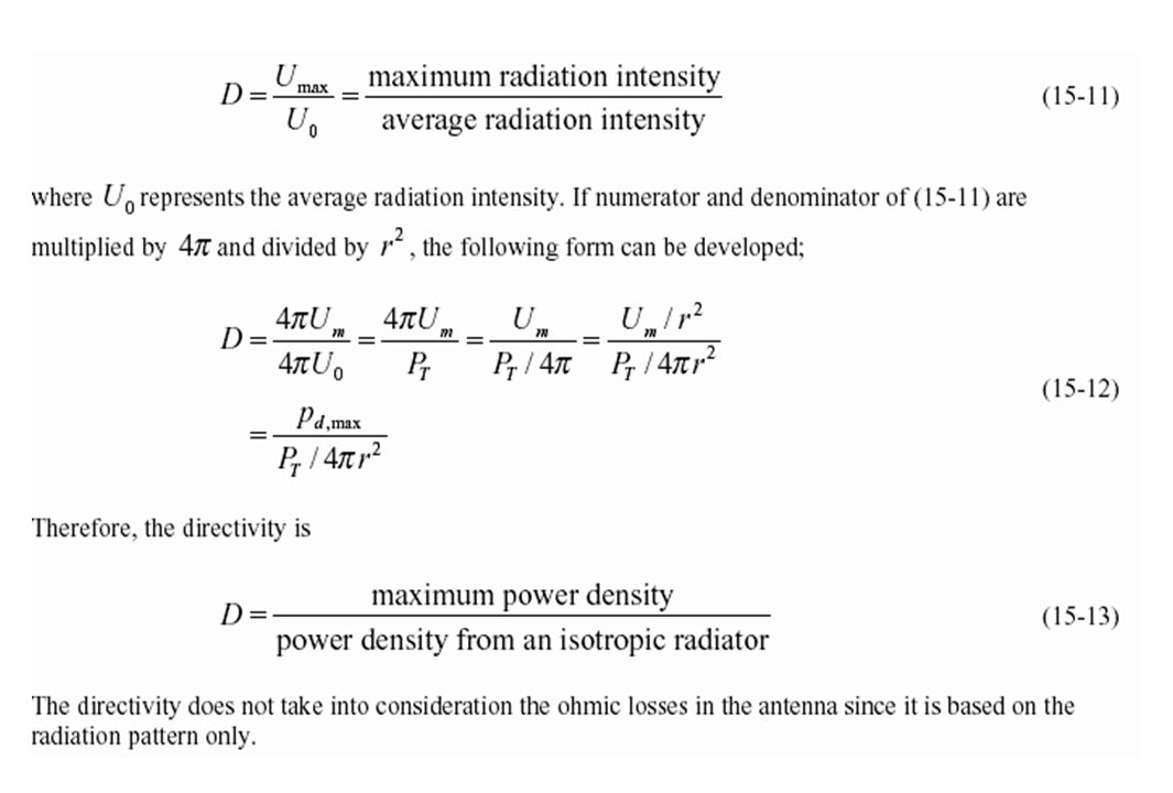
94. 15-6 Directivity and Antenna Gain
There are two commonly employed terms used to describe the radiation characteristics of an antenna:
directivity and antenna gain.
Directivity is a characteristic of the radiation pattern of an ideal lossless antenna while the antenna gain includes the ohmic losses of the antenna physical structure.
Directivity : The directivity D of an antenna is defined from the radiation pattern as

96. Antenna Gain
Antenna gain is defined as the ratio of the maximum radiation intensity Umax to the maximum radiation intensity Uref from a reference antenna with same power input to the antenna.
The difference between directivity and gain is that directivity is referenced to the power radiated by the antenna, while gain is referenced to the power delivered by the transmission line to the antenna. Therefore, gain is always less than or equal to directivity, the difference being the power dissipated in the antenna ohmic losses.
Normally, antenna gain is expressed as a power ratio and is usually specified in decibels as

97. The value of gain depends on the gain of the reference antenna
The value of gain depends on the gain of the reference antenna. It is important to know what reference has been used for the antenna gain. Two of the common references are as follows:
1. a lossless isotropic antenna, in which the radiation intensity is uniform over the sphere surrounding the antenna, i. e., all 4 steradians
2. a reference dipole.
The lossless isotropic antenna is a theoretical concept and has never been realized in practice, while the dipole is readily available.

98. Antenna measurements of gain are usually referenced to a standard dipole for low-gain antennas or to a standard-gain horn for higher-gain antennas.
Accurate theoretical calculations of the gain referenced to a lossless isotropic antenna are possible for both the standard dipole and the standard-gain horn.
The absolute gain of a standard half-wave dipole with respect to an isotropic radiator is or 2.16 dB
Dbi = Dbd +2,16

100. Exercise in dbd &dbi
dBd (dB dipole) The gain an antenna has over a dipole antenna at the same frequency. A dipole antenna is the ….. ., least gain practical antenna that can be made.
The term dBd generally is used to describe antenna gain for antennas that operate under 1GHz (1000Mhz), ( manufacturers calibrate their equipment using a simple dipole antenna as the standard. Then they replace it with the antenna they are testing. The difference in gain (in dB) is reference to the signal from the dipole).

101. dBi (dB isotropic) Unfortunately, an isotropic antenna cannot be made in the real world, but it is useful for calculating theoretical fade and System Operating Margins. The gain of Microwave antennas (above 1 GHz) is generally given in dBi. A dipole antenna has 2.14 dB gain over a 0 dBi isotropic antenna.
So if an antenna gain is given in dBd, not dBi, …… 2.15 to it to get the dBi rating.
For example, if an antenna has 5 dBd gain, it would have ………. dBi gain.

102. Antenna Efficiency
It depends on the ohmic losses of the antenna. It is the ratio of the total power radiated from the antenna / the power delivered to the antenna from the transmission line.
It is also equal
where D and G are the absolute values of directivity and gain.

103. 1- An antenna is transmitting 200 W of power
1- An antenna is transmitting 200 W of power. The maximum power density at a distance of 10 km is mW/m2. Determine the directivity of the antenna.

104. 2- An antenna with a directivity of 16 dB is transmitting a power of 1 kW. Determine the maximum power density at a distance of 50 km from the antenna.

105. 3-An antenna has an efficiency of 95% and the directivity is 33 dB
3-An antenna has an efficiency of 95% and the directivity is 33 dB. Determine the antenna gain in dB.

106. 15-7 Effective Area of an RX Antenna (capture area )
. It is the area by which the power density in watts per unit of area is multiplied to obtain power in watts delivered to the load.
It is close to the physical area of the antenna.
The effective antenna area Ae of the parabolic reflector is given by

108. 15-8 Polarization
By definition, the polarization of an electromagnetic wave propagating in free space is the orientation of the electric field intensity vector relative to the surface of the earth.
There are two basic types of polarization: linear and elliptical.

109. In linear polarization, the electric vector does not change orientation as it travels away from an observer : 2 Types : H& V
In elliptical polarization, the electric vector rotates as it travels away from an observer, and the tip of the electric vector traces an ellipse : sense here mean Clockwise and anticlockwise.

110. An antenna transmits vertical, horizontal, right-hand (RH) circular, or left-hand (LH) circular polarization depending on the antenna design and orientation.
There is a significant cross-polarization loss of approximately 30 dB.
This loss also occurs in case of cross sens rotation in circularly polarized antennas.
This characteristic is used to provide polarization diversity in communication systems.

111. Polarization Requirements for Various Frequencies
wave type
Ground wave
Sky waves
Direct waves (including satellite)
frequency Band
Low & Medium
Short waves
VHF , UHF,SHF
Polarization possible to be used
Vertical
Vertical or Horizontal
Vertical orHorizontal
Polarization practically to be used
 Horizontal
Why
The earth is fairly good conductor ,short out Eh
a) Less auto and electro ignition, b) Less building absorption c) More simple support antenna structure
No ionosphere entry or reflexion

112. 15-9 Antenna Impedance and Radiation Resistance
when it is excited by an appropriate AC source The antenna acts like an a complex impedance to the source providing power to it
Z = R + jX
This impedance can be measured by an appropriate RF bridge .

113. Antenna Impedance
Ideally, it should be purely resistive R at the frequency of operation and equal to the characteristic impedance of the line connected to it.
Self Impedance of the isolated antenna
If an antenna is isolated from ground and any other surrounding objects, this impedance is the self-impedance of the antenna & at the resonance it is purely resistive ( Z= R +j0)

114. Mutual impedance of the antenna.
When other antennas, objects, or ground is near the antenna, the currents flowing in these objects have an influence on the antenna impedance.
The antenna impedance is then determined both by the self-impedance of antenna and by a mutual impedance between the antenna and the nearby objects.

115. Radiation Resistance
The radiation resistance is the real part of the complex antenna impedance of a lossless antenna. It is equal to
Where : - Prad is the amount of this energy leaving a sphere surrounding the antenna per unit of time is the power radiated by the antenna.
- Irms is the rms value of the antenna current magnitude at the input terminals of the antenna.

116. Example : An antenna has an rms current of 3 A flowing into the antenna, and it is transmitting 1 kW of power. Determine the radiation resistance of the antenna.
Solution
The radiation resistance is determined from (15-29).

117. Basic antenna types : - Simple Dipoles - Folded Dipoles
- Antennas Above a Ground Plane
- Monopole Antenna
- Waveguides and horn antennas
- Parabolic antennas

118. High Frequency Antennas
Simple Dipoles
- Folded Dipoles
- Antennas Above a Ground Plane
- Monopole Antenna

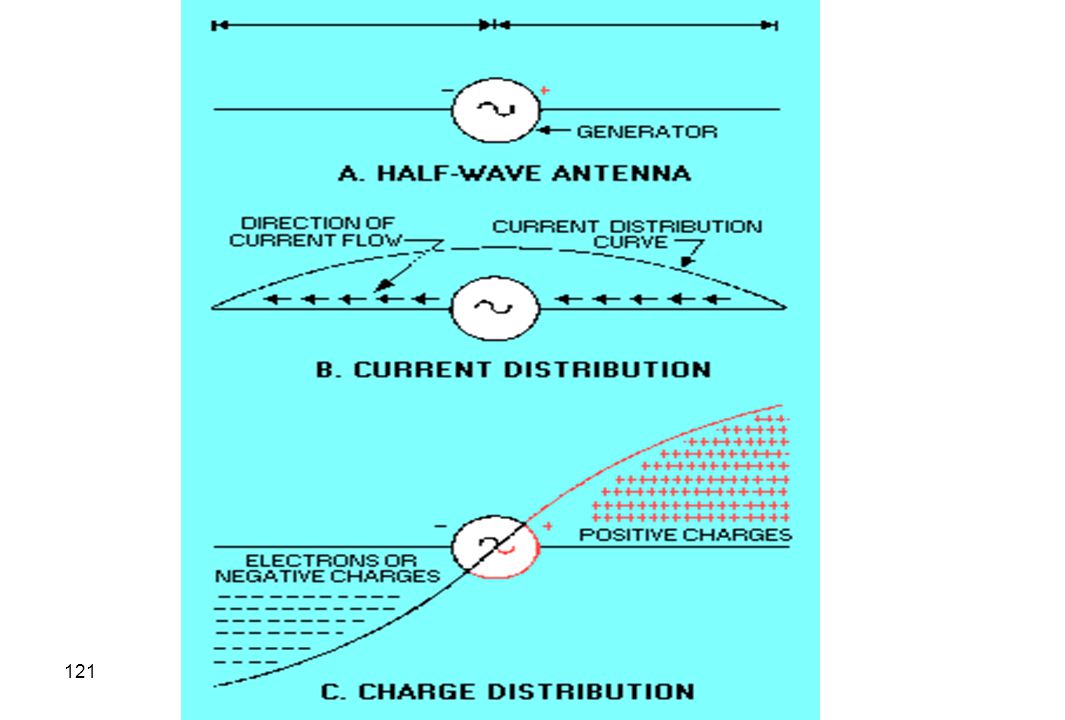
119. Dipoles
One of the simplest and most commonly used antennas is the half-wave dipole, formed from a two-wire parallel transmission line as shown in The following figure.
Starting with an open-ended line, which has a voltage maximum at the open end and a voltage minimum back from the open end, the two conductors are bent 90o from the transmission line as illustrated in the Figure.

120. The theoretical length of the antenna is the
Diameter d of the wires is assumed to be much smaller than the length, and the spacing D at the feed point must be small compared with the length.

122. Practically Mounted dipole

123. Input Impedance of Dipole
A voltage minimum and a current maximum occur at the feed point, which means that the impedance is a minimum at that point.
The actual value of the impedance of the half-wave dipole is j .

124. The reactive component can be eliminated by tuning the antenna, which is accomplished by shortening the length by about 5% from 0.5 to 0.475, corresponding to approximately 95% of the theoretical length.
When properly tuned, the half-wave dipole has an impedance of 73  resistive, which for a lossless dipole is the radiation resistance of the antenna.

125. The dipole is a balanced antenna and must, therefore, be fed by a balanced transmission line.
Since the most common transmission line providing the best impedance match is coaxial cable, a balun must be used to properly connect a coaxial cable to a dipole.

126. Radiation Patterns
The E plane and H plane radiation patterns of the half-wave dipole were shown in the following Figure as examples of patterns.
The E plane pattern is like a doughnut with two maxima broadside to the dipole and a null at both ends of the dipole.
The 3-dB beamwidth is 78o. The isotropic power gain or directivity for a lossless /2 dipole is folds or 2.16 dB.

128. As shown in the Figure , the polarization of the dipole is parallel to the dipole.
The H plane pattern is illustrated in the Figure and is a uniform circular pattern with a constant gain for an angle of 360o about the dipole.

129. Effective Area
The effective area of a dipole can be determined from the isotropic gain and is
for f= 98MHz(=3m) ; Ae =1.218m2

130. Folded Dipole
A folded dipole is constructed from a /2 length of
300- twin-lead transmission line (see figure).
The combination of the 73- self-impedance of the dipole and the mutual impedance from the parallel conductor connected at both ends increases the antenna impedance of the folded dipole to 280 .
Therefore, the folded dipole is a balanced 280- antenna, which closely matches the 300- twin-lead balanced transmission line.

132. Practically mounted Folded antenna

133. The folded dipole is the perfect antenna for stations that require a truly professional antenna for their broadcasting. One powerful advantage of a folded dipole antenna is that is has a wide bandwidth, in fact a one octave bandwidth. This is the reason it was often used as a TV antenna for multi channel use. Folded dipole antennas were mainly used in conjunction with Yagi antennas.
No tuning or adjustment is needed for any frequency on the band which makes this antenna the only one to use if you plan to move your transmitters frequency often.

134. Specifications for the folded professional antenna
Max Power Input
300 Watts
Impedance
50 Ohms
Gain
0dBd
VSWR
Better than 1:1.5 ( MHz)
Frequency Range
MHz (No Tune)
Connector
N-Type Female
Dimension
1600mm(height) x 150mm x 35mm
Weight
2kg

136. 15-11 Antennas Above a Ground Plane
A ground plane is a uniform good ground plane surface beneath an antenna- constructed from good conductors, or at some frequencies, the earth acts as a good ground plane.
Electromagnetic fields cannot exist in a perfect conductor, and any wave incident upon a perfect conductor will be reflected.

137. Figure illustrates this situation
Figure illustrates this situation. To satisfy the boundary condition that no tangential component of electric field can exist there, the reflected wave will be shifted in phase by 180o.
A concept known as image theory is used to determine the characteristics of an antenna above a ground plane.

138. The reflected wave is like a direct wave from an identical antenna located within the ground plane the same distance from the boundary as the real antenna is above the ground plane.
This situation is illustrated in the following Figure.
The image antenna is similar to an image formed in a mirror at optical frequencies.

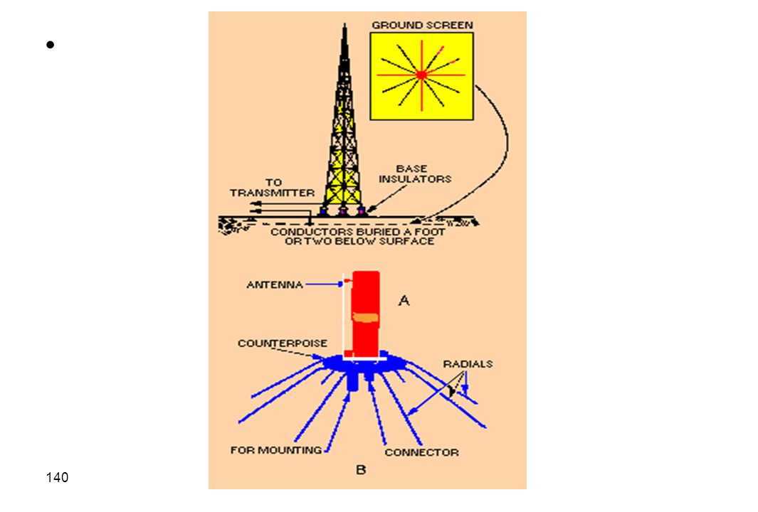
141. Monopole Antenna
An important and commonly used antenna is the /4 monopole antenna on a ground plane as shown in the Figure.
This is an unbalanced antenna since the feed point is between the monopole and ground and it has vertical polarization.
The radiation resistance is 36.5 , and the antenna impedance has a reactive component of 21 j . When the monopole is located close to the ground plane, the image antenna forms a dipole as shown in the previous Figure .

142. The E plane radiation pattern is that of a /2 dipole with only one-half of the pattern above the ground plane.
The ground plane can be achieved either by a grounded metal disc or by radial wires as shown in the following Figure.
The roof of a vehicle such as a car or truck can form a ground plane for a /4 monopole.