2. Why do Americans earn more and produce more than Europeans?
Compared to the average European, the average American works longer hours, produces more, earns more, and faces a labor market with less unemployment.
Why? 2

3. 8 Potential GDP and the Natural Unemployment Rate
CHAPTER CHECKLIST
When you have completed your study of this chapter, you will be able to
1 Explain what determines potential GDP.
2 Explain what determines the natural unemployment rate.
Notes and teaching tips: 4, 15, 38, 44, and 53.
To view a full-screen figure during a class, click the red “expand” button.
To return to the previous slide, click the red “shrink” button.
To advance to the next slide, click anywhere on the full screen figure.
To enhance your lecture, check out the Lecture Launchers, Land Mines, and Class Activities in the Instructor’s Manual.

4. MACROECONOMIC APPROACHES AND PATHWAYS
The Three Main Schools of Thought
The three main approaches to macroeconomics are based on three schools of thought:
Classical macroeconomics
Keynesian macroeconomics
Monetarist macroeconomics
Don’t skip over the Lucas wedge and Okun gap material in the “Eye On the U.S. Economy.”

5. MACROECONOMIC APPROACHES AND PATHWAYS
Classical Macroeconomics
According to classical macroeconomics, the market economy works well and delivers the best available macroeconomic performance.
Aggregate fluctuations are a natural consequence of an expanding economy with rising living standards.
Government intervention can only hinder the ability of the market to allocate resources efficiently.

6. MACROECONOMIC APPROACHES AND PATHWAYS
Classical macroeconomic fell into disrepute during the 1930s, which was a decade of high unemployment and stagnant production throughout the world.
Great Depression is a decade (the 1930s) of high unemployment and stagnant production throughout the world economy.
Classical macroeconomics predicted that the Great Depression would end but gave no method for ending it more quickly.

7. MACROECONOMIC APPROACHES AND PATHWAYS
Keynesian Macroeconomics
According to Keynesian macroeconomics, the market economy works is inherently unstable and the requires active government intervention to achieve full employment and sustained economic growth.
John Maynard Keynes, in his book “The General Theory of Employment, Interest, and Money,” began this school of thought.
Keynes’ theory was that too little consumer spending and investment lead to the Great Depression.

8. MACROECONOMIC APPROACHES AND PATHWAYS
Keynes’ solution to depression and high unemployment was increased government spending.
But Keynes predicted that his policy aimed at curing unemployment in the short term might increase it in the long term.
This prediction became reality during the 1960s and 1970s, when inflation exploded, growth slowed, and unemployment increased.
The global recession of 2008–2009 and fear of another great depression revived interest in Keynesian ideas.

9. MACROECONOMIC APPROACHES AND PATHWAYS
Monetarist Macroeconomics
According to monetarist macroeconomics, the classical view of the world is broadly correct, but in addition to fluctuations that arise from the normal functioning of the an expanding economy, fluctuations in the quantity of money also bring the business cycle.
A slowdown in the growth rate of money brings recession and a large decrease in the quantity of money brought the Great Depression.

10. MACROECONOMIC APPROACHES AND PATHWAYS
Milton Friedman was the most prominent monetarist.
The view that monetary contractions are the sole source of recessions is held by few economists today.
But the view that the quantity of money plays a role in economic fluctuations is accepted by all economists and is part of today’s consensus.

11. Today’s Consensus MACROECONOMIC APPROACHES AND PATHWAYS
Each of the earlier schools provides insights and ingredients that survive in today’s consensus.
Classical macroeconomics provides the story of the economy at or close to full employment.
But the classical approach doesn’t explain how the economy performs in the face of a major slump in spending.

12. MACROECONOMIC APPROACHES AND PATHWAYS
Keynesian macroeconomics takes up the story in a recession or depression.
When spending is cut and the demand for most goods and services and the demand for labor all decrease, prices and wage rates don’t fall but the quantity of goods and services sold and the quantity of labor employed do fall and the economy goes into recession.
In a recession, an increase in spending by governments, or a tax cut that leaves people with more of their earnings to spend, can help to restore full employment.

13. MACROECONOMIC APPROACHES AND PATHWAYS
Monetarist macroeconomics elaborates the Keynesian story by emphasizing that a contraction in the quantity of money brings higher interest rates and borrowing costs, which are a major source of cuts in spending that bring recession.
Increasing the quantity of money and lowering the interest rate in a recession can help to restore full employment.
And keeping the quantity of money growing steadily in line with the expansion of the economy’s production possibilities can help to keep inflation in check and can also help to moderate the severity of a recession.

14. The Road Ahead MACROECONOMIC APPROACHES AND PATHWAYS
Another component of today’s consensus is the view that the long-term problem of economic growth is more important than the short-term problem of recessions.
Even a small slowdown in economic growth brings a huge cost in terms of a permanently lower level of income per person.
The Road Ahead
We follow the new consensus and begin with an explanation of what determines potential GDP and the pace at which it grows.

15. 8.1 POTENTIAL GDP
Potential GDP is the value of real GDP when all the economy’s factors of production are fully employed.
We produce the goods and services that make up real GDP by using factors of production: labor and human capital, physical capital, land, and entrepreneurship.
At any given time, the quantities of human capital, physical capital, land, entrepreneurship, and the state of technology are fixed.
But the quantity of labor is not fixed.
Students sometimes understand the definition of potential GDP but have a hard time seeing it in practice. You may want to spend some time comparing the United States to Europe using the Eye on the Global Economy box Potential GDP in the United States and Europe. If you talked about global differences in unemployment in chapter 21, discussing higher unemployment benefits and less flexible labor markets for France, Germany, and Italy, you can now use this information again to highlight how this determines differences in potential GDP. Use the Eye on the Global Economy box to describe the labor market differences. Mention that the higher unemployment benefits in Europe reduce the opportunity cost of job search. Together with differences in attitudes toward leisure, Europeans work an average of 28 hours per week compared to Americans’ 34 hours per week. Then link this discussion to the calculation of potential GDP. This will help to cement ideas that potential GDP is not some mythical number that is the same for each economy but that it depends on the underlying differences across countries, which include both labor market differences and productivity differences.

16. 8.1 POTENTIAL GDP
The quantity of labor employed depends on the choices of people and businesses.
So real GDP produced depend on the quantity of labor employed.
To describe the relationship between real GDP and the quantity of labor employed, we use a relationship called the production function.

17. The Production Function
8.1 POTENTIAL GDP
The Production Function
Production function is a relationship that shows the maximum quantity of real GDP that can be produced as the quantity of labor employed changes and all other influences on production remain the same.

18. 8.1 POTENTIAL GDP Figure 8.1 shows the production function.
100 billion hours of labor can produce $9 trillion of real GDP at point A.

20. 8.1 POTENTIAL GDP
200 billion hours of labor can produce $13 trillion of real GDP at point B.
300 billion hours of labor can produce $16 trillion of real GDP at point C.
The production function PF is a limit to what is attainable.

21. 8.1 POTENTIAL GDP
The production function is a boundary between the attainable and the unattainable.
The production function displays diminishing returns: The tendency for each additional hour of labor employed to produce successively smaller additional amounts of real GDP.

22. The Labor Market 8.1 POTENTIAL GDP
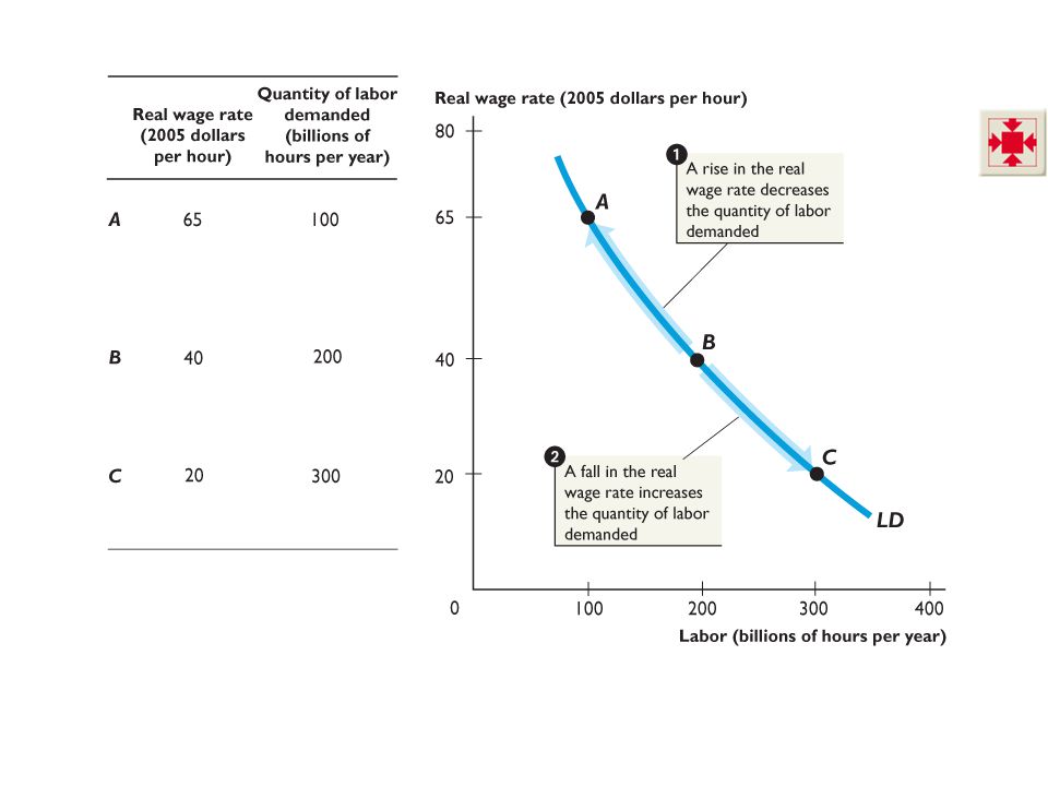
The Demand for Labor
Quantity of labor demanded is the total labor hours that all the firms in the economy plan to hire during a given time period at a given real wage rate.

23. 8.1 POTENTIAL GDP
Demand for labor is the relationship between the quantity of labor demanded and real wage rate when all other influences on firms’ hiring plans remain the same.
The lower the real wage rate, the greater is the quantity of labor demanded.

24. 8.1 POTENTIAL GDP
Figure 8.2 shows the demand for labor.

26. 8.1 POTENTIAL GDP
1. If the real wage rate rises from $40 to $65 an hour, the quantity of labor demanded decreases.

27. 8.1 POTENTIAL GDP
2. If the real wage rate falls from $40 to $20 an hour, the quantity of labor demanded increases.

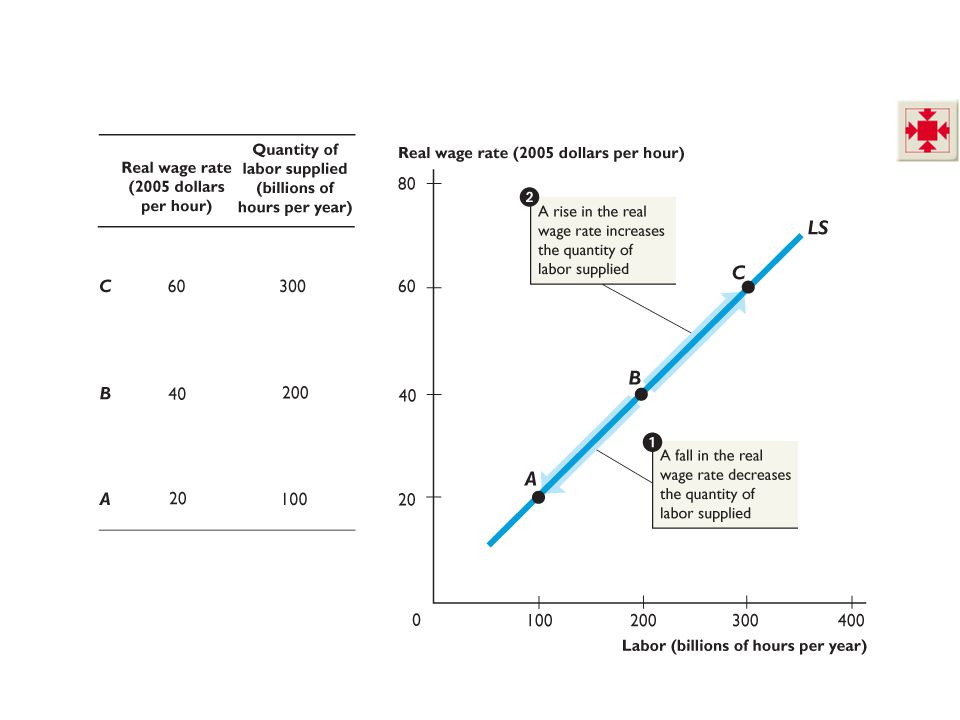
28. 8.1 POTENTIAL GDP
The Supply of Labor
Quantity of labor supplied is the number of labor hours that all the households in the economy plan to work during a given time period and at a given real wage rate.
Supply of labor is the relationship between the quantity of labor supplied and the real wage rate when all other influences on work plans remain the same.

29. 8.1 POTENTIAL GDP
Figure 8.3 shows the supply of labor.

31. 8.1 POTENTIAL GDP
1. If the real wage rate falls from $40 to $20 an hour, the quantity of labor supplied decreases.

32. 8.1 POTENTIAL GDP
2. If the real wage rate rises from $40 to $60 an hour, the quantity of labor supplied increases.

33. 8.1 POTENTIAL GDP
The quantity of labor supplied increases as the real wage rate increases for two reasons:
Hours per person increase as the real wage rate increases.
The labor force participation rate increases as the real wage rate increases.

34. 8.1 POTENTIAL GDP Labor Market Equilibrium
A rise in the real wage rate eliminates a shortage of labor by decreasing the quantity demanded and increasing the quantity supplied.
A fall in the real wage rate eliminates a surplus of labor by increasing the quantity demanded and decreasing the quantity supplied.
If there is neither a shortage nor a surplus, the labor market is in equilibrium.

35. 8.1 POTENTIAL GDP Figure 8.4(a) shows labor market equilibrium.
1. Full employment occurs when the quantity of labor demanded equals the quantity of labor supplied.
2. Equilibrium real wage rate is $40 an hour.
3. Full-employment quantity of labor is 200 billion hours a year.

37. 8.1 POTENTIAL GDP Full Employment and Potential GDP
When the labor market is in equilibrium, the economy is at full employment.
When the economy is at full employment, real GDP equals potential GDP.

38. 8.1 POTENTIAL GDP Figure 8.4(b) shows potential GDP.
1. When the full-employment quantity of labor is 200 billion hours a year,
This is a good place to try to get students to start thinking about the current position of the economy and then tie back to this in future chapters. Ask students to think about what they know about the economy regarding GDP and unemployment. Ask them whether they think that the unemployment rate is above or below the natural rate of unemployment in the United States (in other words, is unemployment high or low right now relative to where it is usually at–have students think about discussions of unemployment they might have heard on the news or at home to make some conjectures here). Use this discussion to determine whether the United States is at potential GDP, or perhaps above it or below it.
2. Potential GDP is $13 billion.

40. Why Do Americans Earn More and Produce More than Europeans?
EYE on U.S. POTENTIAL GDP
Why Do Americans Earn More and Produce More than Europeans?
The quantity of capital per worker is greater in the United States than in Europe.
U.S. technology, on the average, is more productive than European technology.
These differences between the United States and Europe mean that U.S. labor is more productive than European labor. 40

41. Why Do Americans Earn More and Produce More than Europeans?
EYE on U.S. POTENTIAL GDP
Why Do Americans Earn More and Produce More than Europeans?
Because U.S. labor is more productive than European labor, U.S. employers will pay more for a given quantity of labor than European employers will pay.
1. The U.S. demand for labor in lies to the right of the European demand for labor. 41

42. Why Do Americans Earn More and Produce More than Europeans?
EYE on U.S. POTENTIAL GDP
Why Do Americans Earn More and Produce More than Europeans?
2. Higher European income taxes and unemployment benefits mean that the European supply of labor lies to the left of the U.S. supply.
3. Americans work longer hours than Europeans.
4. The equilibrium real wage rate in the United States is higher than in Europe. 42

43. Why Do Americans Earn More and Produce More than Europeans?
EYE on U.S. POTENTIAL GDP
Why Do Americans Earn More and Produce More than Europeans?
Because U.S. labor is more productive than European labor, the U.S. production function, lies above the European production function.
3. Americans work longer hours than Europeans.
5. Potential GDP is higher in the United States than in Europe. 43

44. 8.2 THE NATURAL UNEMPLOYMENT RATE
So far, we’ve focused on the forces that determine the quantity of labor employed.
Now we look at what determine the unemployment rate when the economy is at full employment?
To understand the amount of frictional and structural unemployment that exists at the natural unemployment rate, economists focus on two fundamental causes of unemployment:
Job search
Job rationing
Ask your students how many of them would take a job 2,000 miles away if it paid 5 percent more (10 percent, 20 percent more). Explain that this is another kind of labor market rigidity. That is, as people marry and have children they begin to settle down in a community. They might have relatives close by and have developed long‐standing relationships. It is difficult to simply pull up stakes and move half way across the country to take a job offer. Another important point to get across is to convince students not to think about the unemployment rate as being a single number. Unemployment rates vary substantially across states and regions.
You might get your students to use the BLS Web site to find the unemployment rate in selected major metropolitan areas and note the large variation.
Pose the question: if job prospects are so good for some of the cities listed, then why aren’t workers migrating to them and away from the areas where labor market prospects are comparatively poorer like New York or Chicago?
The answer: not everyone is willing to immediately pull up stakes and move.

45. 8.2 THE NATURAL UNEMPLOYMENT RATE
Job Search
Job search is the activity of looking for an acceptable vacant job.
The amount of job search depends on
Demographic change
Unemployment benefits
Structural change

46. 8.2 THE NATURAL UNEMPLOYMENT RATE
Demographic Change
An increase in the proportion of the population that is of working age brings an increase in the entry rate into the labor force and an increase in the unemployment rate.
This factor increased the unemployment rate during the 1970s and decreased it during the 1980s.

47. 8.2 THE NATURAL UNEMPLOYMENT RATE
Unemployment Benefits
An unemployed person who receives no unemployment benefits faces a high opportunity cost of job search and has an incentive to keep job search brief.
An unemployed person who receives generous unemployment benefits faces a lower opportunity cost of job search and has an incentive to search for longer.

48. 8.2 THE NATURAL UNEMPLOYMENT RATE
Structural Change
Labor market flows and unemployment are influenced by the pace and direction of technological change.
Technological change can bring a structural slump, as it did during the 1970s.
As some industries contracted in the 1970s, labor turnover increased, job search increased, and the natural unemployment rate increased.
Technological change can bring a structural boom, as it did during the 1990s.

49. 8.2 THE NATURAL UNEMPLOYMENT RATE
Job Rationing
Job rationing occurs when the real wage rate is above the full-employment equilibrium level.
The real wage rate might be set above the full-employment equilibrium level for three reasons:
Efficiency wage
Minimum wage
Union wage

50. 8.2 THE NATURAL UNEMPLOYMENT RATE
Efficiency Wage
If a firm pays only the going market wage, employees have no incentive to work hard because they know that even if they are fired for shirking, they can find another job at a similar wage rate.
So some firms pay an efficiency wage.
Efficiency wage is a real wage rate that is set above the full-employment equilibrium wage rate to induce greater work effort.

51. 8.2 THE NATURAL UNEMPLOYMENT RATE
The Minimum Wage
If the government sets a minimum wage above the equilibrium wage rate, unemployment results.
Union Wage
Labor unions operate in some labor markets and agree a wage with employers.
Union wage is a wage rate that results from collective bargaining between a labor union and a firm.

52. 8.2 THE NATURAL UNEMPLOYMENT RATE
Job Rationing and Unemployment
The above-equilibrium real wage rate decreases the quantity of labor demanded and increases the quantity of labor supplied.
If the real wage rate is above the full-employment equilibrium level, the natural unemployment rate increases.

53. 8.2 THE NATURAL UNEMPLOYMENT RATE
Figure 8.5 shows how job rationing increases the natural unemployment rate.
An efficiency wage rate
1. Decreases the quantity demanded—job rationing.
Where is unemployment in the demand-supply diagram? Thoughtful students often ask about the relationship between the (microeconomic-based) labor demand-labor supply model and unemployment. They can’t “see” any unemployment in labor market equilibrium. Where is it, they want to know.
Explain that in the labor market, people use their time in two economically productive ways: work and job search.
Working is supplying labor and this is the activity that the labor demand-supply model shows. The labor demand-supply model does not determine the quantity of job-search. People undertake job-search because workers have imperfect knowledge about available jobs and firms have imperfect information about job seekers.
During the time spent on full-time job search, people are unemployed.
Only if there were no uncertainty would the supply of job search (and unemployment) be zero. In such a case, a person out of work would not need to search for a new job. He or she would simply report to the new job on the day the worker knew that the job started! Thus, workers would never be unemployed because they would never search for jobs. Clearly, this happy state of affairs is not a description of reality.
2. Increases the quantity of labor supplied.
3. Increases the natural unemployment rate.