Download presentation
Presentation is loading. Please wait.

1
Magnetic dynamos in accretion disks Magnetic helicity and the theory of astrophysical dynamos Dmitry Shapovalov JHU, 2006

2
Outline - Turbulence and magnetic fields in astrophysics - Dynamo problem - How the dynamo works: - old theory: mean-field dynamo - new theory: role of magnetic helicity - How can we learn is it true? - Results: what we did so far - Future: what else can be done

3
Cosmic magnetic fields Crucial: stellar and solar activity, star formation, pulsars, accretion disks, formation and stability of jets, cosmic rays, gamma-ray bursts Probably crucial: protoplanetary disks, planetary nebulae, molecular clouds, supernova remnants Role is unclear: stellar evolution, galaxy evolution, structure formation in the early Universe Probably unimportant: planetary evolution

4
Cosmic magnetic fields - Polarization of radiation: orientation || (Zweibel & Heiles, 1997, Nature, 385, 131) Orion
 Orion")
5
Cosmic magnetic fields - Polarization of radiation: orientation || - Zeeman splitting:

6
Cosmic magnetic fields - Polarization of radiation: orientation || - Zeeman splitting: - Synchrotron radiation: intensity, polarization NGC 2997

7
Cosmic magnetic fields - Polarization of radiation: orientation || - Zeeman splitting: - Synchrotron radiation: intensity, polarized - Faraday rotation: for lin. polarized waves: Han et al., 1997, A&A 322, 98

8
Cosmic magnetic fields - Polarization of radiation: orientation || - Zeeman splitting: - Synchrotron radiation: intensity, polarized - Faraday rotation: for lin. polarized waves: - direct measurements for the Sun, solar wind & planets TRACE satellite, 1998-2006

9
Turbulence Observed / predicted in: - convective zones of the stars and planets - stellar wind and supernova explosions - interstellar medium, both neutral and ionized - star forming regions - accretion disks - motion of galaxies through IGM Freyer & Hensler, 2002 Vieser & Hensler, 2002

10
Turbulence Observed / predicted in: - convective zones of the stars and planets - stellar wind and supernova explosions - interstellar medium, both neutral and ionized - star forming regions - accretion disks - motion of galaxies through IGM Freyer & Hensler, 2002 Vieser & Hensler, 2002

11
Origin of the cosmic magnetic fields 1. Origin of the weak initial local or uniform seed field 2. Amplification of the seed field

12
Origin of the cosmic magnetic fields 1. Origin of the weak initial local or uniform seed field 2. Amplification of the seed field Theories range from fluctuations of hypermagnetic fields during the time of decoupling of electroweak interations (come together with baryonic asymmetry of the Universe), to various battery effects, which produce macroscopic seed fields on a continuing basic up to our time. One example is a Poynting-Robertson effect: M.Harwit, Astrophysical Concepts
, to various battery effects, which produce macroscopic seed fields on a continuing basic up to our time. One example is a Poynting-Robertson effect: M.Harwit, Astrophysical Concepts.")
13
Origin of the cosmic magnetic fields 1. Origin of the weak initial local or uniform seed field 2. Amplification of the seed field

14
Origin of the cosmic magnetic fields 1. Origin of the weak initial local or uniform seed field 2. Amplification of the seed field local (chaotic) seed field strong intermittent field, with a scale of the largest eddies Small-scale dynamo
 seed field strong intermittent field, with a scale of the largest eddies Small-scale dynamo.")
15
Origin of the cosmic magnetic fields 1. Origin of the weak initial local or uniform seed field 2. Amplification of the seed field uniform (large-scale) seed field local (chaotic) seed field strong intermittent field, with a scale of the largest eddies Small-scale dynamo Large-scale dynamo strong field with a largest scale available,
 seed field local (chaotic) seed field strong intermittent field, with a scale of the largest eddies Small-scale dynamo Large-scale dynamo strong field with a largest scale available,.")
16
Systems with large-scale dynamos - Earth, Jupiter, some other planets and their satellites - the Sun - accretion disks - some spiral galaxies - giant molecular clouds

17
Earth - turbulence is driven by temperature gradient in liquid outer core - large-scale shear is given by Earth rotation - Re ~, Rm ~ 350, resistive timescale ~ years - B ~ 3 gauss (at CMB), exists for billions of years Radial component of the Earths field at core-mantle boundary (CMB) G.Rüdiger, The Magnetic Universe, 2004
, exists for billions of years Radial component of the Earths field at core-mantle boundary (CMB) G.Rüdiger, The Magnetic Universe, 2004")
18
Accretion disks - protostellar disks - close binaries - active galactic nuclei (AGNs) Illustration, D.Darling T Tauri YSO, image by NASA
 Illustration, D.Darling T Tauri YSO, image by NASA")
19
Accretion disks - protostellar disks - close binaries - active galactic nuclei (AGNs) Illustration, NASA
 Illustration, NASA")
20
Accretion disks - protostellar disks - close binaries - active galactic nuclei (AGNs) Quasar PKS 1127-145, image by ChandraIllustration, NASA/ M.Weiss
 Quasar PKS , image by ChandraIllustration, NASA/ M.Weiss")
21
Accretion disks - large-scale shear is given by Keplerian motion, - angular momentum, i.e. it should be removed in some way when - ordinary viscosity is too small - turbulent viscosity requires turbulence and even then it will be small

22
Accretion disks - large-scale shear is given by Keplerian motion, - angular momentum, i.e. it should be removed in some way when - ordinary viscosity is too small - turbulent viscosity requires turbulence and even then it will be small - large-scale poloidal magnetic field can remove angular momentum from the system:

23
Accretion disks - large-scale shear is given by Keplerian motion - even if Keplerian flow is stable over radial perturbations, in presence of vertical magnetic field turbulence can exist via MRI (magnetorotational instability, Balbus & Hawley, 1991) - MRI can drive the growth of azimuthal field, i.e. large-scale seed for a dynamo process Now we should explain how dynamo works

24
Dynamo theory

25
Macroscopic magnetohydrodynamic (MHD) framework: scale >> m.f.path, plasma scales (Larmor & Debye radii) velocity << sound speed (for incompressibility)
 framework: scale >> m.f.path, plasma scales (Larmor & Debye radii) velocity << sound speed (for incompressibility)")
26
Induction equation: Solar flares: ; Galaxies: => magnetic fields are frozen into liquid, B cant change its topology from small scales to the large ones => for dynamos

27
Mean-field electrodynamics In differentially rotating object: radial seed field is stretched along the direction of rotation => azimuthal field grows To keep azimuthal field growing one needs to maintain radial component in some way: -effect (Moffatt, 78; Parker, 79)
")
28
- large-scale part - turbulent e.m.f.

29
- kinetic helicity: - symmetry should be broken in all 3 directions for - doesnt depend on any magnetic quantitities (, B ) - small-scale quantity: direct cascade - not a conserved quantity in MHD, even for negligibly small - cant support dynamo for a long time: magnetic back-reaction cancels all kinetic helicity at large scales (there is no preferred orientation for spirals) - -effect contradicts to simulations (Hughes & Cattaneo, 96, Brandenburg, 01) Mean-field theory have to be revised
 - small-scale quantity: direct cascade - not a conserved quantity in MHD, even for negligibly small - cant support dynamo for a long time: magnetic back-reaction cancels all kinetic helicity at large scales (there is no preferred orientation for spirals) - -effect contradicts to simulations (Hughes & Cattaneo, 96, Brandenburg, 01) Mean-field theory have to be revised")
31
Magnetic helicity

32
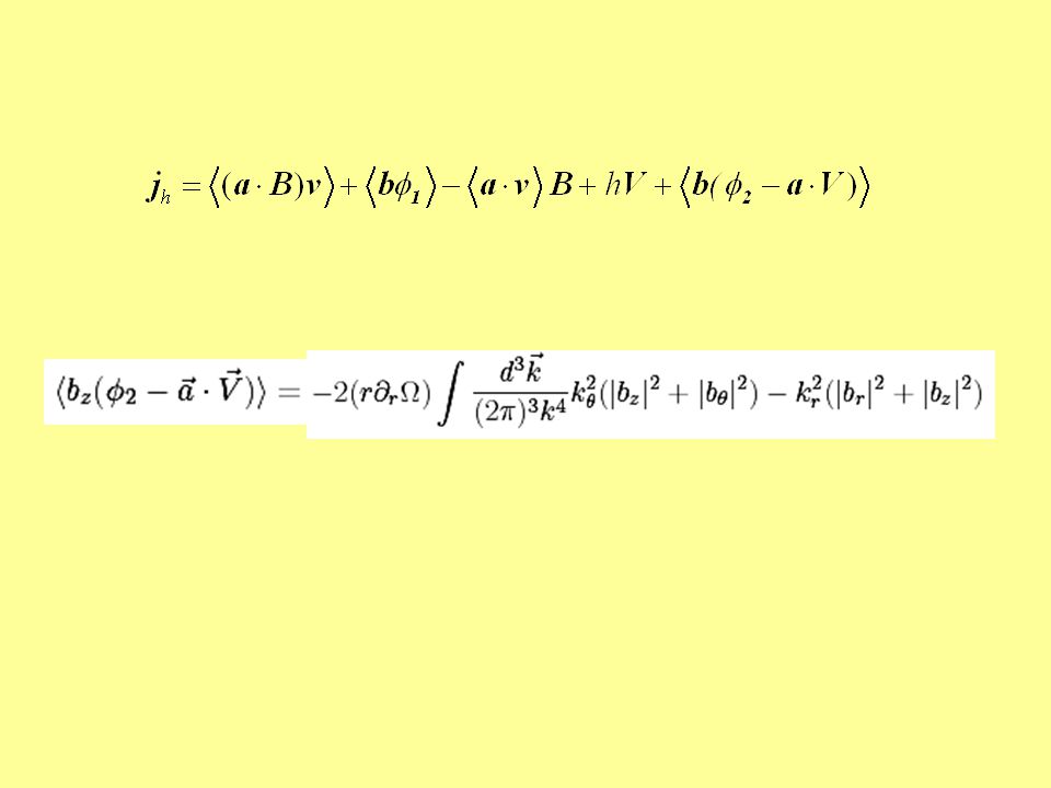
- is conserved quantity in MHD: Magnetic helicity - helicity current - H is the only integral in 3D, which has inverse cascade: cant dissipate at small scales, remains at large ones, where resistivity is negligible, i.e. exists for a time bigger than dissipative timescale

33
- transfer of magnetic helicity between scales Mean-field dynamo depends on the transfer of magnetic helicity between scales where - turbulent e.m.f. (In mean-field treory )
.")
35
Simulations General features: - incompressible 3D MHD - pseudospectral ( E, H - conserved, unlike in spatial code) - periodic box ( H is gauge invariant) - resolution: from 64^3 to 1024^3 - timescale up to 100 eddy turnover times - both OpenMP & MPI parallel versions available
 - periodic box ( H is gauge invariant) - resolution: from 64^3 to 1024^3 - timescale up to 100 eddy turnover times - both OpenMP & MPI parallel versions available")
36
Simulations Dynamo-specific features: - = (to simplify) - turbulence is driven by external random (gaussian) forcing - forcing has N components with variable spectral properties - forcing correlation time is variable - forcing has both linearly and circularly polarized components (for helicity injection into the turbulence) - divF =0
 - turbulence is driven by external random (gaussian) forcing - forcing has N components with variable spectral properties - forcing correlation time is variable - forcing has both linearly and circularly polarized components (for helicity injection into the turbulence) - divF =0")
37
Simulations Dynamo-specific features: - turbulence is driven by external random (gaussian) forcing - forcing has N components with variable spectral properties - forcing correlation time is variable - forcing has both linearly and circularly polarized components (for helicity injection into the turbulence) - divF =0 - forcing is usually set at some fixed small scale (to simulate real systems)
 forcing - forcing has N components with variable spectral properties - forcing correlation time is variable - forcing has both linearly and circularly polarized components (for helicity injection into the turbulence) - divF =0 - forcing is usually set at some fixed small scale (to simulate real systems)")
38
Simulations Dynamo-specific features: - forcing correlation time is variable - forcing has both linearly and circularly polarized components (for helicity injection into the turbulence) - divF =0 - forcing is usually set at some fixed small scale (to simulate real systems) - initial large scale shear and weak seed field:
 - divF =0 - forcing is usually set at some fixed small scale (to simulate real systems) - initial large scale shear and weak seed field:")
39
Simulations Dynamo-specific features: - forcing has both linearly and circularly polarized components (for helicity injection into the turbulence) - divF =0 - forcing is usually set at some fixed small scale (to simulate real systems) - initial large scale shear and weak seed field ( |B o | << |V o | ): - l.-s. shear is maintained const for anisotropy / against dissipative decay

40
Results

41
Energy evolution sm.scale forcing: kx/k = 1 Ro ~ 1, timespan ~ 10 e.t. _____________

42
Energy spectra sm.scale forcing: kx/k = 1 Ro ~ 1, timespan ~ 10 e.t. |k| Magnetic energy spectra Kinetic energy spectra time

43
BxBy Bz B total time |k| Magnetic field spectra sm.scale forcing: kx/k = 1 Ro ~ 1, timespan ~ 10 e.t.

44
|k| time Bx By B total Bz Magnetic field spectra sm.scale forcing: kx/k = 1 | Bo | ~ | Vo |, Ro ~ 10, timespan ~ 10 e.t.

45
Evolution of large-scale magnetic energy for different initial large-scale fields timesteps, 5K ~ 1.e.t. Bo = 0.1 Bo = 0.01 Bo = 0.001

46
Evolution of large-scale magnetic energy for timesteps, 5K ~ 1.e.t.

47
Magnetic helicity spectra |k|time

48
Future - next big goal is to prove numerically that turbulent e.m.f. depends on transfer of magnetic helicity between scales (balance formula) - then it is interesting to see how different terms in helicity current influence the dynamo - code: do subgrid modelling in order to expand dynamic range even more (to have everything covered: from large- scale shear to the dissipation scale ) All results we obtained so far already fit well into the helicity-based picture of the large-scale dynamo
 - then it is interesting to see how different terms in helicity current influence the dynamo - code: do subgrid modelling in order to expand dynamic range even more (to have everything covered: from large- scale shear to the dissipation scale ) All results we obtained so far already fit well into the helicity-based picture of the large-scale dynamo.")
49
The end

50
Energy spectra for different forcing spectral distribution Here: ky/k = 0.1 other parameters - real-life _______________________ No dynamo action when kx/k = 0 |k| Magnetic energy spectra Kinetic energy spectra time

51
V, B = large scale v, b = small scale Vo, Bo - initial large- scale fields ______________ Vo = Vx ~ exp(iky) Bo = Bx ~ exp(iky) sm.scale forcing: kx/k = 1 | Bo | << | Vo |, Ro ~ 10 50 BxBy Bz B total time |k|
 Bo = Bx ~ exp(iky) sm.scale forcing: kx/k = 1 | Bo | << | Vo |, Ro ~ BxBy Bz B total time |k|")
52
Balance formula

54
Simulations with real-life parameters Ro ~ 1 in accretion disks, Suns convection zone. Constant large-scale shear (to compensate disipative decay and to maintain non-uniformity in the system). Weak initial magnetic field: |Bo| << |Vo|. We want large scale shear to help in generation of magnetic field from some small seed field. Forcing correlation time ~ eddy turnover time. Small scale turbulence is driven by some instability which saturates when its growth time ~ eddy turnover time.
. Weak initial magnetic field: |Bo| << |Vo|. We want large scale shear to help in generation of magnetic field from some small seed field. Forcing correlation time ~ eddy turnover time. Small scale turbulence is driven by some instability which saturates when its growth time ~ eddy turnover time..")
Similar presentations


![Progress and Plans on Magnetic Reconnection for CMSO For NSF Site-Visit for CMSO May1-2, 2005 1. Experimental progress [M. Yamada] -Findings on two-fluid.](/2/736643/big_thumb.jpg "Progress and Plans on Magnetic Reconnection for CMSO For NSF Site-Visit for CMSO May1-2, 2005 1. Experimental progress [M. Yamada] -Findings on two-fluid.>")


 Fausto Cattaneo Center for Magnetic Self-Organization in Laboratory and Astrophysical Plasmas Chicago 2003.>")


