1. NONLINEAR DYNAMIC
FINITE ELEMENT ANALYSIS IN ZSOIL :
with application to geomechanics & structures
Th.Zimmermann
copyright zace services ltd

2. Far-field BC needed
2-phase medium
Ground motion

3. For time being in Z_Soil: limited structural dynamics
a, or d t

4. with some extensions
analysis by geomod

5. STATICS RECALL

6. STATIC EQUILIBRIUM STATEMENT, 1-PHASE
Boundary value problem
displacement imposed
on u
Equilibrium
12 +(12 /x2)dx2
12 f1
traction imposed
on  
11
11+(11/x1)dx1 x2 x1
dx1
direction 1:
(11/x1)dx1dx2+(12 /x2) dx1dx2+ f1dx1dx2=0
L(u)= ij/xj + fi=0
(Differential equation
of equilibrium)

7. FORMAL DIFFERENTIAL PROBLEM STATEMENT
1-phase,linear or nonlinear)
(equilibrium)
(displ.boundary cond.)
(traction bound. cond.)
Incremental elasto-plastic constitutive equation:
NB: Time is steps

8. Kd=F MATRIX FORM -DISCRETIZATION LEADS TO THE MATRIX FORM….
FOR LINEAR STATICS
Kd=F
( K=stiffness matrix, F=vector of nodal forces
d=vector of nodal displacements)

9. DYNAMICS

10. DYNAMIC EQUILIBRIUM STATEMENT, 1-PHASE
Boundary value problem
displacement imposed
on u
Equilibrium
traction imposed
on 
12 +(12 /x2)dx2
12 f1 
11
11+(11/x1)dx1 x2 x1
dx1
direction 1:
(11/x1)dx1dx2+(12 /x2) dx1dx2+ f1dx1dx2=0
L(u)= ij/xj + fi=0

11. FORMAL DIFFERENTIAL PROBLEM STATEMENT
Deformation(1-phase):
(equilibrium)
(displ.boundary cond.)
(traction bound. cond.)
(initial conditions)
Incremental elasto-plastic constitutive equation:
NB: Time is real

12. Kd=F Ma(t)+[Cv(t)]+Kd(t) =F(t) COMPARING MATRIX FORMS STATICS
(linear case)
Kd=F
We obtain
(Linear system size:
Ndofs=Nnodes x NspaceDim,
-d=nodal displacements
-F=nodal forces)
DYNAMICS
(linear case)
Ma(t)+[Cv(t)]+Kd(t)
=F(t)
where
We obtain
(Linear system size:
Ndofs=Nnodes x NspaceDim,
But 3xNdofs unknowns)
optional

13. SOLUTION TECHNIQUES
-MODAL ANALYSIS
-FREQUENCY DOMAIN ANALYSIS
both essentially restricted to linear problems
-DIRECT TIME INTEGRATION
appropriate for a fully nonlinear analysis

14. DIRECT TIME INTEGRATION (linear case)…a)
Using Newmark’s algorithm :
At each time step, solve:

15. DIRECT TIME INTEGRATION (linear case)…b)

16. Ma(t)+Cv(t)+Kd(t)=F(t) >>>>
MATRIX FORMS
STATICS
(linear case)
Kd=F
DYNAMICS
(linear case)
Ma(t)+Cv(t)+Kd(t)=F(t)
>>>>
at any tn+1
we have an equivalent static problem
K*dn+1=F*n+1
an+1=………… vn+1=…………

18. NEWMARK IS A 1-STEP ALGORITHM
All information to compute solution at time tn+1,
is in solution at time tn , restart is easy

19. NUMERICAL ( ALGORITHMIC) DAMPING CAN EXIST
and varies with parameters (γ ,β) ● ●
Newmark(0.6,0.3025) ● ●
HHT ● ● ● ●
Newmark(0.5,0.25) ● ● ● ● ● ● ●
IT MAY BE WANTED OR NOT

20. DISCRETIZATION APPROXIMATES HIGH FREQUENCIES
Exact sol.:
Filtering of high
frequencies may
be desirable

21. HHT Hilber-Hughes-Taylor α method
HHT filters high frequencies without damping low frequencies

22. NUMERICAL ( ALGORITHMIC) DAMPING CAN EXIST
and varies with parameters (γ ,β) ● ● ● ●
HHT(-0.3) ● ● ● ● ● ● ● ● ● ● ●
IT MAY BE WANTED OR NOT

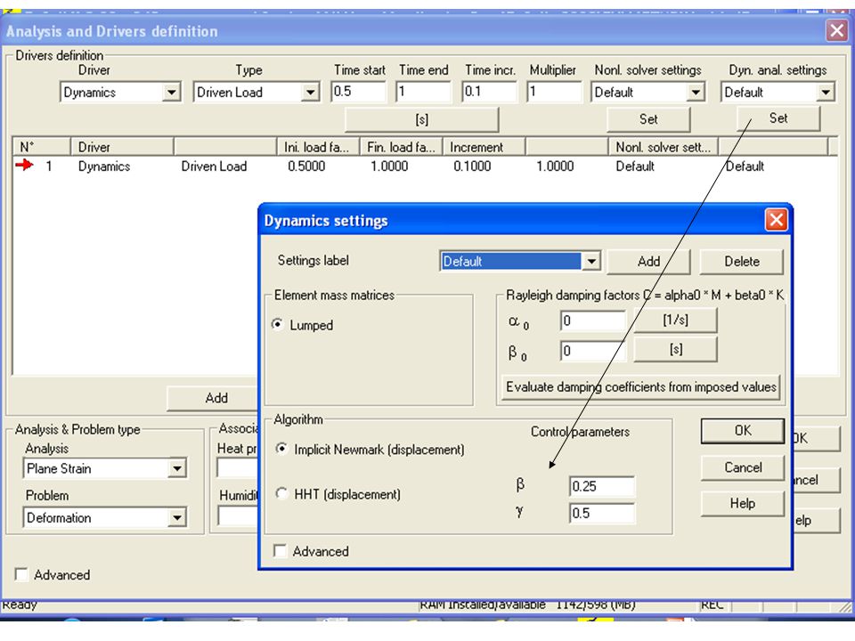
23. Algorithmic data for Newmark …or HHT(under CONTROL/AN..

24. Mass can be CONSISTENT (as obtained by FEM)
or LUMPED (concentrated at (some) nodes)
Only lumped masses are available in ZSOIL
Lumped masses tend to lead to underestimate frequencies

25. Lumped masses tend to lead to underestimate frequencies:
ILLUSTRATION

26. C=αM+βK is RAYLEIGH DAMPING
RAYLEIGH DAMPING a)
Recall: Ma(t)+Cv(t)+Kd(t)=F(t)
C=αM+βK is RAYLEIGH DAMPING
α,β:constants
This form of damping is not representative of physical reality, in general. Its success is due to the fact that it
maintains mode decoupling in modal analysis

27. RAYLEIGH DAMPING b):
PARENTHESIS ON MODAL ANALYSIS

28. RAYLEIGH DAMPING d) COMPARING THE MODAL EQUATION
WITH THE 1DOF VISCOUSLY DAMPED OSCILLATOR
YIELDS:

29. RAYLEIGH DAMPING e)

30. RAYLEIGH DAMPING f)
this can be plotted

31. 2 (ω,ξ) pairs are used to define α0,β0 in ZSOIL

32. NONLINEAR DYNAMICS

33. CONSTITUTIVE MODEL: ELASTIC-PERFECTLY PLASTIC
1- dimensional  E  y
this problem is non-linear

34. FROM LOCAL TO GLOBAL NONLINEAR RESPONSE

35. SOLUTION OF LINEARIZED PROBLEM, static case
Nonlinear problem to solve d
Linearize at , w. Taylor exp.
hence the following algorithm:
i: iteration
n: step

36. THE PROBLEM IS NONLINEAR & THEREFORE
NEEDS ITERATIONS
tends to 0
Fn+1 Fn
i: iteration
n: step d

37. d Fn
Fn+1
NEWTON- RAPHSON & al.
ITERATIVES SCHEMES d Fn
Fn+1
KTo
2.Constant stiffness,use KTo
till
i: iteration
n: step
3.Modified NR, update KT opportunistically, each step e.g.,till
1.Full NR, update KT at each
step & iteration, till
4. BFGS, “optimal”secant
scheme

38. TOLERANCES ITERATIVE ALGORITHMS

39. Ma(t)+Cv(t)+N(d(t))=F(t)
MATRIX FORMS
STATICS
(nonlinear case)
N(d)=F
DYNAMICS
(nonlinear case)
Ma(t)+Cv(t)+N(d(t))=F(t)
>>>>
(e.g.)

40. DIRECT TIME INTEGRATION (nonlinear case)
Using Newmark’s algorithm (or Hilber’s):
At each time step, solve:

41. Ma(t)+Cv(t)+N(d(t))=F(t) or Ma(t)+N(d,v)=F(t)
MATRIX FORMS
STATICS
(nonlinear case)
N(d)=F
DYNAMICS
(nonlinear case)
Ma(t)+Cv(t)+N(d(t))=F(t) or
Ma(t)+N(d,v)=F(t)
>>>>at any tn+1,
we have an equivalent static problem
N*(dn+1)=F*n+1
an+1=………… vn+1=…………
Like for linear case

42. SEISMIC INPUT a
>>>
equilibrium
>>Fin+Fdamp+Fel = Fext

43. SEISMIC INPUT b
yields

44. Time-history