2. A phenomenon is random if individual outcomes are uncertain but there is nonetheless a regular distribution of outcomes in a large number of repetitions.
Randomness requires a long series of independent trials.
The probability of any outcome of a random phenomenon is the proportion of times the outcome would occur in a very long series of independent repetitions. That is, probability is a long-term relative frequency of independent repetitions.

3. Thus, the chance of something gives the percentage of time it is expected to happen, when the basic process is done over & over again, independently & under the same conditions.

4. A probability model is based on independent trials
A probability model is based on independent trials. Besides independent trials, it requires:
A list of possible outcomes of the random phenomenon: the sample space.
A probability for each outcome or set of outcomes—each event—of the random phenomenon.

5. Think of the probability model as a box model.
See Freedman et al., Statistics.

6. E.g., someone has a set of 10 cards consisting of three cards with #1, one card with #2, two cards with #4, two cards with #7, one card with #8, & one card with #10. The cards are put in a box & mixed well.
We make 5 draws from the box. After each draw, the drawn card is replaced & the cards are remixed. For each draw, what are the chances of drawing the following numbers: 1, 2, 3, 4, 5, 6, 7, 8, 9, 10?

7. Card # Probability (for each card drawn) 1 .30 2 .10 4 .20 7 .20 8 .10
Sum of event probabilities=1.0

8. How did we compute the probabilities for the box model?

9. We did so:
By making a list of the possible outcomes of the random phenomenon: the sample space; &
By assigning a probability for each outcome (or set of outcomes) of the random phenomenon—for each event.

11. Create the variables . input cardnum prob 1 .3 2 .1 4 .2 7 .2 8 .1
10 .1
end

12. . gr bar prob, over(cardnum)

13. To be valid, the assigned probabilities must be premised on independent, random draws (i.e. independent, randomly drawn observations).

14. In the previous example about card values, consider the set of cards as a population.
What we did, then, was draw a sample from that population.
What was the basis of the mean of the sample drawn?

15. It was the sample’s particular set of draws from the population’s sample space of events (i.e. card values) & the probability attached to each event.

16. . gr bar prob, over(cardnum)
How to do a probability histogram (which in Stata can done via the ‘bar’ graph command)?
. gr bar prob, over(cardnum)
Histogram: breaks a quantitative continuous or discrete variable’s range of values into intervals & displays the count or percent of observations falling into each interval; density (continuous) or frequency (discrete) histograms.
Bar graph: displays the counts or percentages of the components of a categorical variable.

17. . gr bar prob, over(cardnum)

18. Probability Rules
(1) The probability of an event A is between 0 & 1. That is, chances are between 0% & 100%.
The summed probability of all events in a sample space=1. That is, P(S) = 1.

19. (3) The complement of any event A is the event that A does not occur (e.g., live vs. die). Then P(Ac) = 1 - P(A).
That is, the chance of something equals 100% minus the chance of the opposite thing.

20. (4) Two events are disjoint (i. e
(4) Two events are disjoint (i.e. mutually exclusive) if they have no outcomes in common & thus can never occur simultaneously (e.g., the probability of being single or married). Then P(A or B) = P(A) + P(B).
(5) If events A & B are independent, then P(A and B) = P(A)P(B).
E.g., P(divorced and male).
Why is independence a tricky issue?

21. Remember that in the previous chapter we began moving from descriptive statistics to inferential statistics.
We’re about to examine methods of inferential statistics in greater depth, based on probability principles.

22. The following, then, is about using one or more samples to obtain statistics, which in turn we’ll use to estimate parameters.
In particular, we’ll obtain sample means & sample standard deviations, which in turn we’ll use to estimate a population’s mean.

23. We’ll begin to apply probability principles toward this objective by defining the following:
Random variable
Expected value of a random variable

24. We’ll also do so by introducing a modification to the standard deviation, which will become the standard error.
This modification will divide a sample’s standard deviation by the square root of the sample size-n.

25. With this modification, what varies is the mean of samples from the population mean. How is the meaning of standard error, then, different from that of standard deviation?
Understanding this difference, as we’ll see, is fundamental to understanding the difference between descriptive & inferential statistics.

26. And again, what makes all of this possible?
The principles of probability.

27. Random Variable
A random variable is a variable whose value is a numerical outcome of a random phenomenon.

28. A discrete random variable X has a finite number of possible values
A discrete random variable X has a finite number of possible values. The probability distribution of X lists the values & their probabilities.
E.g., number of suicides in Miami-Dade last year; number of votes by candidate in Mexico’s presidential election; number of members per household in South Africa; number of housing types in Miami-Dade; number of persons by gender in FIU.

29. A continuous random variable X takes values in an interval of numbers
A continuous random variable X takes values in an interval of numbers. Its probability distribution is described by a density curve. The probability of any even is the area under the density curve & above the values of X that make up the event.
E.g., age, weight, cholesterol level, temperature; the proportion of adults that opposes abortion rights for women; the proportion of immigrants that sends remittances to home countries.

30. Because any density curve describes an assignment of probabilities, density distributions are probability distributions.

31. Means, Variances & Standard Deviations of Discrete Random Variables
The mean of a random value X is called the expected value of X: a weighted, long-term average in which each outcome is weighted by its probability.

32. Expected value of a discrete random variable:
The previous card example.
Votes per candidate.
Number of persons per household.

33. Let’s calculate the expected value for the previously discussed playing cards example:
Card Number Probability (for each draw)
Each card value times its probability, summing the results.

34. Variance of a discrete random variable: (each value – the mean)squared, summing the results
Standard deviation of a discrete random variable: square root of the variance.

35. Why do we refer to the expected value of a random variable instead of its mean?

36. Because we’re moving from descriptive statistics to inferential statistics.
That is, from merely describing one or more samples to using them to make inferences about a population.

37. In this regard, expected value indicates that the mean of a random variable is a long-term outcome of its weighted probabilities.
It is the value that we’d expect to obtain if we could measure an entire population.
When we draw a sample, what determines the sample mean? How does this pertain to the expected value?

38. The purpose of using the expected value of a random variable—the outcome of its weighted probabilities over the long term—becomes clearer when we turn our attention to the Law of Large Numbers.

39. Statistical Estimation & the Law of Large Numbers
We’ve seen how sample means vary from sample to sample.
If the sample mean of a statistic rarely captures the parameter & varies from sample to sample, why is it nonetheless a reasonable estimate of the parameter?

40. Because when based on a random sample of independent observations:
The sample mean is an unbiased estimator of the population mean; &
We can reduce its variability by increasing the sample size.

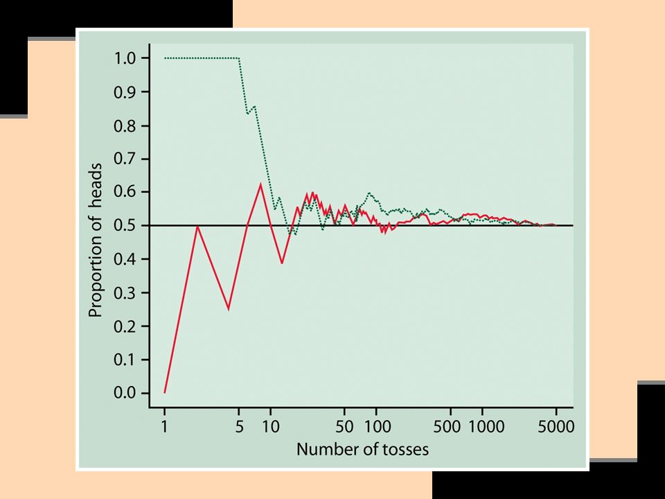
41. Another reason: The Law of Large Numbers.
If we keep adding observations to our random sample of independent observations (i.e. if we keep making the sample size-n larger), the sample mean of a statistic is guaranteed to get as close as we wish to the parameter & to stay that close.

42. That is, if we make a sample-n large enough, eventually its mean outcome gets close to the population mean & stays close.
This holds for any population, not just for some special class such as normal distributions.

44. Based on the Law of Large Numbers, the mean of a large number of independent observations is stable & predictable.

45. The Law of Large Numbers versus the ‘Law of Small Numbers’:
The Law of Large Numbers: probability operates over the very long run.
The ‘Law of Small Numbers’: in our daily lives we tend to behave as if probability operated in the short run.

46. Means & Variances of a Random Variable
Rules for means of a random variable
Rules for variances of a random variable (& take the square root to compute standard deviation).

47. Rules for Means of Random Variables
If X & Y are random variables, then the mean of X + Y = mean of X + mean of Y
. mean of 7 dents per car + mean of 12 scratches per car = mean of 19 imperfections per car
. mean household size of Dominicans in Miami + mean household size of Jamaicans in Miami = mean D + mean J

48. And if X is a random variable, then multiplying the mean of X by a constant = multiplying each randomly selected observation by a constant.

49. E.g., 3.23*mean income = 3.23*each randomly selected income observation
The former is a new random variable that is based on a linear transformation of the latter.

50. Addition Rule for Variances
If X & Y are independent random variables, then:
variance X+Y=variance X + variance Y
variance X – Y = variance X + variance Y
Why? Because combining two variables in any way adds their variation together.
X & Y are independent if rXY = 0

51. E.g., the mean income of Salvadorans in Miami + the mean income of Haitians in Miami.
The variance, & standard deviation, of their combined incomes.
Key question: Are the Salvadoran & Haitian incomes independent of each other? If not, see Rule 3 for variances (page 330).

52. Let’s not lose sight of what we’re doing:
By using both the expected value of the sample mean of a random variable & its standard deviation divided by the square root of sample size-n (i.e. the standard error): we’re moving from descriptive statistics to inferential statistics.
That is, instead of just describing one or more samples, we’re now using the random samples of size-n to make inferences about a population.

53. What makes such inference possible
What makes such inference possible? The principles of probability, including:
The fact that the sample mean is an unbiased estimator of the population mean & can be made less variable by increasing sample size-n;
& The Law of Large Numbers.

54. The rules of probability assure us that one or more random samples of independent observations of size-n will give us sample means that are reasonably accurate estimates of a parameter.

55. What kind of statistics should be used if a study involves not a sample but rather a population?
Descriptive statistics, not inferential statistics, should be used in this instance.
The reason is that there are no sampling-based uncertainties involved when analyzing a population.

56. Before analyzing a statistic, always ask:
Is the statistic drawn from a random sample of independent observations?
If this premise is not reasonably met, then the use of inferential statistics is invalid.

57. Summary What does probability mean?
What does random mean?
What does probability mean?
What does a probability model require?

58. What are the rules of probability?
What is a random variable? What are its two basic types?

59. Why do we use the expected value of a random variable?
What’s an expected value of a random variable, & how is it computed?
How are the variance & standard deviation of the expected value computed?
Why do we use the expected value of a random variable?

60. What is the Law of Large Numbers? What is the ‘Law of Small Numbers’?
Why is the sample mean of a statistic a reasonable estimate of a parameter?
What is the Law of Large Numbers? What is the ‘Law of Small Numbers’?

61. What are the rules for means of a random variable?
What are the rules for variances of a random variable? How do they pertain to the standard deviation of a random variable?
If we have measures for a population or if we don’t have a random sample, can we use inferential statistics?