Download presentation
Presentation is loading. Please wait.

2
Inventory analysis has always been of concern to top management
Inventory analysis has always been of concern to top management. In many companies, inventory is one or the most expensive and important assets, representing as much as 40 percent of the total invested capital in an industrial organization. Because of the large Investment and the importance to the overall functioning of the firm, it is crucial that good inventory management be practiced. On one hand, companies will try to reduce the cost of inventory by reducing amounts of inventory on hand. On the other hand, however, it is realized that customer dissatisfaction can be increased significantly due to low inventory levels and stock outs. Inventories are needed to achieve workable systems of production, distribution, and marketing of goods.

3
Regardless of the complexity of inventory decisions and their associated mathematical models, only two important decisions must be made concerning any current or potential Item in inventory: When to place an order for an item. How much of that item is to be ordered. To state the problem in simple terms, a manager must decide "when" and "how much" to order rot any particular item. The major objective or the inventory decision is to minimize the total inventory cost, which is comprised of five components: Cost of the items. Cost of ordering. Cost of carrying, or holding, inventory. Cost of safety stock. Cost of stock outs.

4
The inventory models discussed in this unit assume that demand and lead time are known and constant and that quantity discounts are never given. When this is the case, the most significant costs arc the cost of placing an order and the cost at holding inventory items over a period of time. Hence, in making inventory decisions, it will be the overall objective to minimize the sum of the carrying costs and the ordering costs. One of the most common inventory decisions is to determine the quantity to order (economic order quantity, or EOQ) that will minimize the ordering cost and the carrying cost. As the quantity ordered increases, the total number of orders placed per year will decrease, Thus, as the quantity ordered increases, the annual ordering cost will decrease. But as the order quantity increases, the currying cost will also increase, owing to the larger average inventories that the firm will have to maintain.
 that will minimize the ordering cost and the carrying cost. As the quantity ordered increases, the total number of orders placed per year will decrease, Thus, as the quantity ordered increases, the annual ordering cost will decrease. But as the order quantity increases, the currying cost will also increase, owing to the larger average inventories that the firm will have to maintain.")
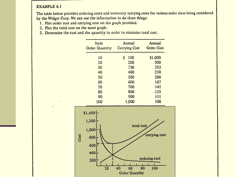
5
The following figure reveals the relationship between the order quantity and the carrying and ordering costs. In addition, the figure shows the total cost and the order quantity that will minimize the total cost. With values for the carrying cost and ordering cost, it is possible to graph a total-cost curve. By plotting the total cost (the sum or the ordering cost and carrying cost), it is possible to determine the minimum inventory cost level, and hence the optimum order quantity.
, it is possible to determine the minimum inventory cost level, and hence the optimum order quantity..")
7
You should note in Example 6
You should note in Example 6.1 that the optimum order quantity occurred at the point where the ordering cost curve and the carrying cost curve intersected. This was not by chance. With the type of cost functions that we will be investigating in this unit, the optimum quantity will always occur at a point where the ordering cost is equal to the carrying cost. This is an important fact to remember. In determining the annual carrying cost, it is convenient to use the average on hand inventory level. In future problems we will multiply the average inventory level times a factor (called inventory carrying capacity per unit) to determine the annual inventory cost. For a constant demand, the inventory usage is constant over time. The inventory level will range from a maximum, which is numerically equal to the order quantity minimum value of 0. Figure 6.2 revels inventory usage over time.
 to determine the annual inventory cost. For a constant demand, the inventory usage is constant over time. The inventory level will range from a maximum, which is numerically equal to the order quantity minimum value of 0. Figure 6.2 revels inventory usage over time.")
8
ECONOMIC ORDER QUANTITY
In Example 6.1 , we pointed out that the optimum order quantity was the point that minimized the total cost, where total cost is the sum of ordering cost and carrying cost. We also indicated that the optimum order quantity was at the point where the ordering cost was equal to the carrying cost. We shall make use of this fact in future problems. Instead of graphically determining optimal inventory levels, let us now develop equations that will directly solve for the optimum. To accomplish this, the following steps need to be performed: I. Develop an expression for ordering costs. 2. Develop an expression for carrying cost. 3. Set ordering cost equal to carrying cost. 4 Solve the equation for tire desired optimum

11
Inventory carrying costs for many business and industries are often expressed as an annual percentage of the unit cost or price. When this is the case, a new variable is introduced. Let I = annual inventory carrying charge as a percentage of price. Then the cost of storing l unit of inventory for the year, Cc, is given by C = IP, where P is the unit price of an inventory item. Q* can be expressed, in this case, as Now that equations for the optimal order quantity, Q*, have been derived, it is possible to solve inventory problems very simple.

12
EXAMPLE 6.3 Sumco, a company that sells pump housings to other manufacturers, would like to reduce its inventory cost by determining the optimal number of pump housings to obtain per order. The annual demand is 1,000 units, the ordering cost is $10 per order, and the average carrying cost per unit per year is $0.50. Using these figures, we can calculate the optimal number of units per order.

13
Total annual cost = order cost + holding cost
The expected number of orders placed during the year, N, and the expected time between orders, T, can also be determined. Expected number of orders, Expected time between orders, T = number of working days in a year divided by N As mentioned earlier in this unit, the total annual inventory cost is the sum of the ordering costs plus the carrying costs. Total annual cost = order cost + holding cost

14
Often the total inventory-cost expression is written to include the actual cost of the material purchased. Since the annual demand in problem 6.4 is assumed to be a known value (8,000 transistors per year) and total price per transistor ($10) is also a known value, total annual cost should include purchase cost. Purchase cost does not depend on the particular order policy found to be optimal, since regardless of how many units are ordered each year, we still incur an annual purchase cost of (D)(P) = (8,000)($l0) = $80,000. (In the next unit, we will discuss the case in which this may not be true-when a "quantity discount" is offered to the customer who orders a certain amount each time.)
 and total price per transistor ($10) is also a known value, total annual cost should include purchase cost. Purchase cost does not depend on the particular order policy found to be optimal, since regardless of how many units are ordered each year, we still incur an annual purchase cost of (D)(P) = (8,000)($l0) = $80,000. (In the next unit, we will discuss the case in which this may not be true-when a quantity discount is offered to the customer who orders a certain amount each time.).")
15
The reorder point, ROP), is given as
RE-ORDER POINTS Now that we have decided "how much" to order, we shall look at a second inventory question, "when to order." In most simple inventory models, it is assumed that receipt of an order is instantaneous. That is, we assume that a firm will wait until its Inventory level fur a particular item reaches zero, place an order, and receive the items in stock immediately. As we all know, however, the time between the placing and receipt of an order, called the "lead time" or delivery time, is often a few days or even a few weeks. Thus, the "when to order" decision is usually expressed in terms of a reorder point, the inventory level at which an order should be placed. The reorder point, ROP), is given as ROP = (demand per day) X (lead time for a new order in days) = d X L The demand per day, d, is found by dividing the annual demand, D, by the number of working days in a year:
, is given as. ROP = (demand per day) X (lead time for a new order in days) = d X L. The demand per day, d, is found by dividing the annual demand, D, by the number of working days in a year:")
16
Example 6.4 Xeinex's demand for transistors is 8,000 per year. The firm operates on a 200~ay working year. On the average, delivery of an order takes 3 working days. The reorder point for transistors is calculated as follows:

17
SENSITIVITY ANALYSIS In the preceding examples and problems we have developed formulas that can be used to solve directly fur the optimum order quantity. These formulas assume that all input values are known with certainty. What would happen, though, if one of the input values in tile EOQ equation changes (for example, the cost of placing an order rises by $5)? The answer is that if any of the values used ii one of the formulas changes, tile optimum order quantity will also change. Determining the effect of these changes is called SENSITIVITY ANALYSIS. One approach to sensitivity analysis is to recalculate the optimum quantity when one of the inputs changes.
 The answer is that if any of the values used ii one of the formulas changes, tile optimum order quantity will also change. Determining the effect of these changes is called SENSITIVITY ANALYSIS. One approach to sensitivity analysis is to recalculate the optimum quantity when one of the inputs changes.")
18
EXAMPLE 6.5 In Example 6.3, we observed that if annual demand for an inventory item is D = 1,000 units, ordering cost is Oc = $10 per order, and carrying cost per unit per year is Cc = $ 0.50, the optimal order quantity, Q*, is found to be 200 units. An in depth study by the Sumco Company reveals, however, that the actual carrying cost for one pump housing per year is not $0.50, as previously estimated, but rather $ How will this affect the optimal order quantity?

19
In order to determine how sensitive the optimal solution is to a change in one of the variables in an equation, it is not always necessary to completely recalculate the order quantity Q* usually, it is possible to determine the effect of a change in the optimal quantity by inspecting the basic EOQ formula. Example 6.6 Let us look at the formula for the "optimum number of units to order, "which was derived in example 6.2. What effect would the following individual changes have on the value of Q4? Ordering cost increases by a factor of 4. Carrying cost increases by a factor of 4. The total number of pieces of inventory sold per year (or the annual demand) decreases by a factor of 9.
 decreases by a factor of 9.")
20
The EOQ formula is given as
The following shortcuts can be used to test the effect of the changes listed. The optimum order quantity will increase by a factor of 2. To see this, we simply replace Oc in the formula by an ordering cost of 4 times that number, (4) (Oc).
 (Oc).")
21
2. The optimal order quality will decrease by a factor of ½
In each of these, we can note that the optimal value of Q* changes by the square root of the change of a variable used in the formula. Thus, in example 6.7, we could have determined that the optimal order quantity would increase by a factor of 2 (of double) because the order cost increased by a value of 4.
 because the order cost increased by a value of 4.")
22
PRODUCTION INVENTORY MODELS
In Unit 6, we assumed that the entire inventory order was received at One time. There are situations1 however, when the firm may receive its inventory over a period of time. For this case, a new model is needed that does not require the instantaneous-receipt assumption. This model is applicable when inventory continuously flows or builds up over a period of time after an order has been placed or when units are produced and sold simultaneously. Under these circumstances, the daily production (or inventory flow) rate and the daily demand rate must be taken into account. Figure 7.1 shows inventory levels as a function of time.
 rate and the daily demand rate must be taken into account. Figure 7.1 shows inventory levels as a function of time.")
23
Because this model is especially suited to the production environment, it is commonly called the production-run-model. It can be used when inventory continuously builds up over time and the traditional economic-order-quantity assumptions can be met. This model can be derived by setting ordering costs equal to carrying costs and solving for the appropriate variable. Example 7.1 starts by developing the expression for carrying cost. It should be noted that setting ordering cost equal to carrying costs does not always guarantee optimal solutions for models more complex than the production-run model. EXAMPLE 7.1 Using the symbols given below, determine the expression for annual inventory carrying cost for the production-run model: Qc=number of pieces per order C = carrying cost per unit per year p = daily production rate d = daily demand rate T = length of the production run (days)
")
24
1. Annual inventory carrying cost
= (average inventory level) x (carrying cost per unit per year) = (average inventory level) x Cc 2. Average inventory level = 1/2 x(maximum inventory level) 3. Maximum inventory level = pt - dt (total produced during the production rate) – (total used during the production run) But Q = total produced = pt, and thus t = Q/p; therefore, maximum inventory level = p (Q/p) – d (Q/p) = Q -d/pQ = Q(1 - d/p) 4.Annual inventory carrying cost (or simply carrying cost) = 1/2 X (maximum inventory level) x Cc = ½ x Q(l -d/p) x Cc
 x (carrying cost per unit per year) = (average inventory level) x Cc. 2. Average inventory level = 1/2 x(maximum inventory level) 3. Maximum inventory level. = pt - dt (total produced during the production rate) – (total used during the production run) But Q = total produced = pt, and thus t = Q/p; therefore, maximum inventory level = p (Q/p) – d (Q/p) = Q -d/pQ = Q(1 - d/p) 4.Annual inventory carrying cost (or simply carrying cost) = 1/2 X (maximum inventory level) x Cc = ½ x Q(l -d/p) x Cc.")
25
EXAMPLE 7.2 Given the following values, solve for the optimum number of units per order. Annual demand, D = 1,000 units Setup cost, Oc = $10 Carrying cost, Cc = $0.5 per unit per year Daily production rate, p = 8 units daily Daily demand rate, d = 6 units daily

26
You may wish to compare this solution with the answer to Problem 6. 5
You may wish to compare this solution with the answer to Problem 6.5. Eliminating the instantaneous receipt assumption, where p = 8 and d = 6, has resulted in Q* increasing from 200 (see Problem 6.5) to 400. Also note that Q * can be calculated when annual data are available. Try the following problem. When annual data are available, Q* can be expressed as
 to 400. Also note that. Q * can be calculated when annual data are available. Try the following problem. When annual data are available, Q* can be expressed as.")
27
BACKORDER INVENTORY MODELS
In previous inventory models, we have not allowed inventory shortages where there was not sufficient stock to meet current demand. There are many situations, however, that suggest that planned shortages or stock outs may be advisable. This is especially true with high inventory carrying costs for expensive items. Car dealerships and appliance stores rarely stock every model for this reason. In the following model, we shall assume that stock outs and back ordering are allowed. This model is called the backorder or planned shortages inventory model. The assumptions for this model are the same as previous models and, in addition3 that sales will not be lost due to a stock out. This model will use the same variables, with the addition of Bc, the cost of back ordering 1 unit for 1 year.

28
Q = number of pieces per order
D = annual demand (units) Cc= carrying cost per unit per year Oc =ordering cost for each order Bc = backordering cost per unit per year S = remaining units after backorder is satisfied Q - S= amount backordered
 Cc= carrying cost per unit per year. Oc =ordering cost for each order. Bc = backordering cost per unit per year. S = remaining units after backorder is satisfied. Q - S= amount backordered.")
29
The total cost must include the cost of being out of stock (or backordering cost)
Tc = ordering cost + carrying cost + backordering cost Calculus is used to solve for Q* and S* once the total cost is expressed using the variables above. The results are as follows: and

30
Example 7.3 Calculate Q* and Q* - S* given the following data D = 20,000 units per year Cc = $ 2 Oc = $ 15 Bc = $ 10

31
QUANTITY DISCOUNT MODEL
To obtain a higher sales volume, many businesses offer reduced product costs for large purchases, typically referred to as quantity discounts. When given the opportunity to purchase large quantities at a reduced product cost, the manager must decide between the economic order quantity and the quantity discount (Qc) The overall approach will be to find which option, QE or QD minimizes total costs, which must now include the product cost. Thus, the objective will be to minimize
 The. overall approach will be to find which option, QE or QD minimizes total costs, which must now include the product cost. Thus, the objective will be to minimize.")
32
Where product cost is usually expressed as annual demand multiplied by the unit price, P, or D X P.
The following steps can be used to decide whether or riot to take the quantity discount. 1. Calculate QE 2. Calculate total cost using QE 3. Calculate total cost using QD. 4. The optimum order quantity will be the quantity with the lower total cost, either QE or QD

33
EXAMPLE 7.4 Given the following data, determine whether or not the quantity discount should be taken D = 500 units Oc = $ 4.9 Cc = $ 1 P = $ 10 If inventory is purchased in lots of 80 units, the discount price will be $8 per unit PD = discount price = $8 QD= discount quantity = 80 units 1. Calculating QE

34
4. Choosing the lowest total cost quantity
4. Choosing the lowest total cost quantity. In this example, the optimal order quantity is Q* = QD= 80 units

Similar presentations