1. Iteration,
the Julia Set,
and the Mandelbrot Set

2. Iteration Terminology
Iteration – to repeat a process over and over.
Iteration rule – the process that will be repeated over and over. (Can be numerical or geometric)
Seed – the place to begin the iteration .
Orbit of the iteration rule – the list of numbers or geometric figures obtained by successively applying the iteration rule to the output of the previous iteration.

3. Linear Iteration
A linear iteration rule is an iteration rule of the form
x → Ax + B where A and B are constants.
An iteration rule is the same thing as a function.

4. Linear Iteration Iteration rule: x → 1 2 x – 2 Seed: 0
Applying the iteration rule produces the following orbit.
0 → –2 → –3 → –3.5 → –3.75 → –3.875 → – → …
The numbers in the orbit are getting closer and closer to –4.
The fate of this orbit is: It approaches –4.

5. Linear Iteration
The seed of an iteration rule is denoted x0, the next term in the iteration is x1, then x2, x3, and so on.
For the orbit
0 → –2 → –3 → –3.5 → –3.75 → …
x0 = 0, x1 = –2, x2 = –3, x3 = –3.5, and so on.

6. Linear Iteration Iteration rule: x → 1 2 x – 2 Seed: x0 = –4
The orbit is
–4 → –4 → –4 → –4 → –4 → …
The orbit stays constant at –4. The number –4 is called a fixed point for this iteration rule.

7. The fixed point can be determined by solving the equation x = Ax + B .
Linear Iteration
The fixed point can be determined by solving the equation x = Ax + B .

8. Linear Iteration Iteration rule: x → 1 2 x – 2 Seed: x0 = 5
The orbit is
5 → 0.5 → –1.75 → –2.875 → – → – → – → …
The orbit of this seed also approaches –4.
The orbit of any seed will approach –4 for this iteration rule.

9. Linear Iteration Iteration rule: x → 2x + 1 Seed: x0 = 0 The orbit is
0 → 1 → 3 → 7 → 15 → 31→ 63 → …
The numbers in this orbit grow larger and larger. This orbit tends to infinity.

10. Linear Iteration
With the iteration rule x → 2x + 1, the orbit of x0 = –2 tends to (negative) infinity since the orbit is
–2 → –3 → –5 → –9 → –17 → –33 → …
The orbit of x0 = –1 is fixed under this iteration rule since x1 = –1.

11. Linear Iteration
For the iteration rule x → –2x, 0 is a fixed point. All other orbits eventually alternate between large positive and large negative values.
The orbit of x0 = 2 under this rule begins
2 → –4 → 8 → –16 → 32 → –64 → 128→ –256 → …
This orbit tends to positive and negative infinity.

12. Linear Iteration
Orbits may also cycle. The orbit of x0 = 4 for the linear iteration rule x → –x + 2 is
4 → –2 → 4 → –2 → 4 → –2 → 4 → …
This orbit is a cycle of period 2 since the orbit repeats every second iteration.

13. Types of Fixed Points
An earlier iteration rule we looked at was x → 1 2 x – 2. We said the fixed point for this rule was –4.
When the seed x0 = 5 was used, the orbit was
5 → 0.5 → –1.75 → –2.875 → – → – → – → …
This orbit tends to –4.
The orbit of 0 also tended to –4.
By iterating the seed x0, it can be shown that any seed will tend to -4.

14. Types of Fixed Points
For the iteration rule x → 1 2 x – 2 , –4 is called an attracting fixed point.
The fixed point for the linear iteration rule x → Ax + B is attracting if all other orbits tend to the fixed point under iteration.

15. Types of Fixed Points
The fixed point of the iteration rule x → 2x + 1 is –1.
The orbit of x0 = 0 tended to infinity.
The orbit of x0 = –2 tended to (negative) infinity.
The fixed point –1 is called a repelling fixed point.
A fixed point for which all other orbits tend to move away from under iteration is a repelling fixed point.

16. Types of Fixed Points
The linear iteration rule x → –x + 2 has a fixed point at x0 = 1, but it is neither attracting nor repelling.
The orbit of x0 = 4 is
4 → –2 → 4 → –2 → 4 → –2 → 4 → …
The orbit of x0 = 7 is
7 → –5 → 7 → –5 → 7 → –5 → 7 → …

17. Types of Fixed Points
If we choose any other seed x0 for the iteration rule
x → –x + 2 then the orbit is
x0 → –x0 + 2 → –(–x0 + 2 ) + 2 = x0.
This orbit begins to cycle after two iterations. This orbit is a cycle of period 2. The fixed point is neither attracting nor repelling, it is a neutral fixed point
There are three types of fixed points, attracting, repelling, and neutral.
The orbit of any seed will approach an attracting fixed point.
The orbit of any seed will approach positive or negative infinity for a repelling fixed point.

18. Quadratic Iteration
A quadratic iteration rule is an iteration rule of the form x → x2 + c where c is a constant.
The fate of the orbit of x → x2 + c depends on the seed and the parameter c.

19. Quadratic Iteration
The orbit of zero, under x → x2 + c, has different fates for different values of c.
When c = 1, the orbit of 0 tends to infinity:
0 → 1 → 2 → 5 → 26 → 677 → …
When c = 0, the orbit remains fixed at 0:
0 → 0 → 0 → 0 → …
When c = −1, the orbit cycles with period 2:
0 → −1 → 0 → −1 → …
When c = −2, the orbit of 0 is eventually fixed:
0 → −2 → 2 → 2 → 2 → …

20. Quadratic Iteration
The orbit of 0 is called the critical orbit of the iteration rule x → x2 + c.
The value 0 is special because the minimum value of
y = x2 + c occurs at x = 0.

21. Quadratic Iteration
Fixed points can also be determined algebraically for quadratic iteration rules.
To find the fixed points, solve the equation
x = x2 + c

22. Quadratic Iteration
Solving the equation x = x2 + c is equivalent to determining the place where the graph of y = x2 + c crosses the diagonal y = x.
The behavior near a fixed point can be determined graphically.
fixed point

23. Quadratic Iteration
The initial seed is a point on the line y = x (or x-axis). The result of an iteration is the y-value on y = x2 + c associated with that x-value. That y-value becomes the next x-value to be iterated.

24. A repelling fixed point
Quadratic Iteration
A repelling fixed point
y = x
y = x2 + c

25. An attracting fixed point
Quadratic Iteration
An attracting fixed point
y = x
y = x2 + c

26. Quadratic Iteration
y = x
y = x
The graph of y = x has a fixed point at x = 0.5.
Appears to be repelling to the right
Appears to be attracting from the left
The fixed point 0.5 is neither attracting nor repelling, it is a neutral fixed point

27. Quadratic Iteration
Orbits of a quadratic iteration may be attracted to a fixed point or they may be repelled from it. Orbits may also cycle or tend to cycles with different periods.

28. Quadratic Iteration
Finding cycles for quadratic iterations algebraically is usually extremely difficult or impossible.
To find the 2-cycle for the rule x → x2 + c, iterate twice
x → x2 + c → (x2 + c)2 + c
And then solve the equation
x = (x2 + c)2 + c
To find the 3-cycle, iterate three times and solve the resulting equation.

29. Complex Linear Iteration
A complex number is a number of the form a + b𝑖.
The magnitude of a complex number is the distance of the complex number from the origin.
The magnitude of a + b𝑖 is a 2 + b 2
The polar angle of a complex number is the angle formed by the positive x-axis and line connecting the complex number to the origin.
The number a is called the real part and b is called the imaginary part.
a + b𝑖 θ

30. Complex Linear Iteration
If a + b𝑖 is a complex number with polar angle θ and magnitude r, then
a = r cos θ
b = r sin θ
a + b𝑖 = r cos θ + 𝑖r sin θ = r(cos θ + 𝑖 sin θ)
This is the polar representation of the complex number a + b𝑖.

31. Complex Linear Iteration
For two complex numbers a + b𝑖 and c + d𝑖:
(a + b𝑖) + (c + d𝑖) = (a + c) + (b + d)𝑖
e(a + b𝑖) = ea + eb𝑖
If a + b𝑖 = r1(cos θ1 + 𝑖sin θ1)
and c + d𝑖 = r2(cos θ2 + 𝑖sin θ2)
(a + b𝑖)(c + d𝑖) = r1r2(cos θ1cos θ2 - sin θ1 sin θ2)
+ 𝑖 r1r2(sin θ1cos θ2 + sin θ2 cos θ1)
(a + b𝑖)(c + d𝑖) = r1r2(cos (θ1+θ2) + 𝑖(sin (θ1+θ2))
Using the polar representation for multiplication gives a result that is more useful when interpreting the results of an iteration.
A trigonometric identity simplifies the product.

32. Complex Linear Iteration
(a + b𝑖)(c + d𝑖) = r1r2(cos (θ1+θ2) + 𝑖(sin (θ1+θ2))
To multiply two complex numbers geometrically, add their polar angles and multiply their magnitudes.

33. Complex Linear Iteration
Iteration rule: x → 2x
Seed: x0 = 1 + 𝑖
The orbit is
1 + 𝑖 → 2 + 2𝑖 → 4 + 4𝑖 → 8 + 8𝑖 → 𝑖 → …
The orbit moves farther and farther away from the origin. This orbit tends to infinity.
1 + 𝑖
2 + 2𝑖
4 + 4𝑖

34. Complex Linear Iteration
Iteration rule: x → 𝑖x
Seed: x0 = a + b𝑖
The orbit is
a + b𝑖 → –b + a𝑖 → –a – b𝑖 → b – a𝑖 → a + b𝑖 → …
Which is a 4-cycle in the complex plane.
(Magnitude is the same, but each point is rotated 90°)
a + b𝑖
–b + a𝑖
–a – b𝑖
b – a𝑖
The multitude of 𝑖 is 1 and the polar angle is 90°. When multiplying by 𝑖, multiply the magnitude by 1 and add 90° to the angle.

35. Complex Linear Iteration
Iteration rule: x → ( 𝑖) x
Seed: 1
1 → 𝑖 → 1 2 𝑖 → − 𝑖 → − → …
This orbit tends to 0. 𝑖
− 𝑖 1
1 2 𝑖
The magnitude of 𝑖 is and the polar angle is 45°. When multiplying by 𝑖 , multiply the magnitude by and rotate the polar angle by 45°.

36. Complex Linear Iteration
Complex iteration rule: x → Ax where A = a + b𝑖
If the magnitude of a + b𝑖 is greater than 1, then when we multiply a number by a + b𝑖, the resulting complex number has greater magnitude.
The orbit of any nonzero number moves further and further from the origin and these orbits tend to infinity.
The origin is a repelling fixed point for this iteration rule.

37. Complex Linear Iteration
Complex iteration rule: x → Ax where A = a + b𝑖
If the magnitude of a + b𝑖 is less than 1, then each successive multiplication results in a complex number with smaller magnitude.
The orbit of any nonzero number moves closer and closer to the origin and these orbits tend to 0.
The origin is an attracting fixed point for this iteration rule.

38. Complex Linear Iteration
Complex iteration rule: x → Ax where A = a + b𝑖
If the magnitude of a + b𝑖 is equal to 1, then the magnitude of the seed is not changed. Multiplication rotates the given point by the polar angle of a + b𝑖.
The origin is a neutral fixed point for this iteration rule.

39. The Squaring Rule Iteration rule: x → x2 y = x2 y = x
Back to the real numbers for a moment.
O and 1 are fixed points for this rule.
Any value less than -1 will go to infinity.
-1 goes to the fixed point 1.
Any number between -1 and 0 goes to the fixed point 0.
Any number between 0 and 1 goes to the fixed point 0.
Any number greater than 1 goes to infinity.
y = x

40. The Squaring Rule Iteration rule: x → x2
If x0 = 0 or 1, the orbit is fixed
If 0 < | x0| < 1, the orbit tends to 0
If | x0| >1, the orbit goes to infinity
If x0 = –1, the orbit is eventually fixed at 1.

41. The Squaring Rule Iteration rule: x → x2 Seed: x0 = r(cos θ + 𝑖 sin θ).
xn = r2n(cos 2nθ + 𝑖 sin 2nθ)

42. The Squaring Rule
Complex squaring iteration does not differ very much from the real case for most seeds.
If r > 1, the orbit tends to infinity since r2n will get larger and larger.
If r < 1, the orbit tends to 0 since r2n will get very small.
If r = 1, the entire orbit lies on the circle of radius 1.

43. The Julia Set
Orbits can be categorized into two types: the orbit tends to infinity or it does not.
If the orbit tends to infinity, the orbit “escapes.”
The collection of all seeds that do not escape is called a filled Julia set.
For the squaring iteration, the filled Julia set consists of all those seeds on and inside the circle of radius 1 centered at the origin.
If r < 1, the orbit tends to 0.
If r = 1, the entire orbit lies on the circle of radius 1.

44. The filled Julia set for the squaring iteration.
The Julia Sets
The filled Julia set for the squaring iteration.

45. The Julia Set
Seeds inside the circle of radius 1 tend to the attracting fixed point at the origin and those that lie on the circle have orbits that stay on the circle forever.
The circle of radius 1 is called the Julia set for this iteration rule.
The Julia set is the boundary between the seeds whose orbits escape and those whose orbits do not.
The boundary is called the Julia set.
The boundary and its interior is the filled Julia set.

46. Julia Sets of Quadratic Iterations
Instead of using the squaring iteration rule, x → x2, the more general quadratic iteration rule, x → x2 + c, can be used.

47. Julia Sets of Quadratic Iterations
It is important to be able to determine the fate of an orbit. If the orbit does not escape, it is in the filled Julia set. If it does escape, it is not in the set.
An orbit will escape under the iteration rule x → x2 + c if its magnitude ever exceeds an escape value.
The escape value is the larger of 2 and the magnitude of the given value of c.
The number 2 is like the value for delta in an epsilon-delta proof. It is something that will make it work out nicely.

48. Julia Sets of Quadratic Iterations
Suppose that xn is a complex number and denotes the nth point along an orbit.
According to the Triangle Inequality
| xn +1| = | xn2 + c | ≥  | xn|2 - |c|
If | xn| > 2, then
| xn|2 - |c| > 2| xn |- |c|.
And if | xn| > |c|, then
2| xn|- |c| > | xn|.
Replace one factor of | xn|2 with 2
The term 2| xn| can be written as | xn|+| xn|. Replace one term with |c|.

49. Julia Sets of Quadratic Iterations
So if | xn | > 2 and | xn | > |c|, then | xn+1| > | xn |.
The sequence is continuously increasing and the orbit of the seed must escape to infinity. 
Therefore, the escape value is the larger of 2 and the magnitude of c.
The escape value is a value that tells you when you can stop iterating, because if the value of xn is larger than this, the orbit will escape to infinity.

50. Julia Sets of Quadratic Iterations
The first step in computing a filled Julia set is to determine the escape value.
Next, divide the complex plane into a grid of complex numbers. Each point on the grid represents a seed.
Compute the orbit of each grid point. If a point on an orbit ever has a magnitude greater than the escape value, then this orbit tends to infinity and is not in the filled Julia set. If that point does not tend to infinity it is in the set.

51. Julia Sets of Quadratic Iterations
Compute the filled Julia set by hand for
x → x2 − 1
Escape value = 2
The value for c is -1. The larger of |-1| and 2 is 2.

52. Julia Sets of Quadratic Iterations
On a TI-83:
Enter the seed, then press enter. (For complex seeds, use on the bottom row.)
Press (This gives x1)
Pressing enter again gives x2.
Continue pressing enter until the magnitude of the answer is > 2 or you have pressed enter 10 times.
If the orbit does not exceed the escape value, plot that point. 𝑖
2nd
ANS x2 − 1
ENTER
Draw Julia Set

53. Julia Sets of Quadratic Iterations

54. Julia Sets of Quadratic Iterations

55. Julia Sets of Quadratic Iterations

56. Julia Sets of Quadratic Iterations
This is sometimes called the fractal rabbit.
It is a rabbit because it has a body and two ears. Ignore the fact that it has two ears at both ends.

57. Julia Sets of Quadratic Iterations
This is a fractal because it is self similar.
Self similarity is a key factor in determining if a figure is a fractal. The other is that it has fractional dimension. This fractal has a dimension of approximately

58. Julia Sets of Quadratic Iterations

59. Julia Sets of Quadratic Iterations
This is fractal dust. Under more iterations, the set of points will becomes smaller and smaller, but there are some points that will never escape.

60. Julia Sets of Quadratic Iterations
The orbit of 0 is called the critical orbit and it plays a role in determining the shape of the filled Julia set.

61. Julia Sets of Quadratic Iterations
x → x2 – 𝑖
x0 = 0
x1 = – 𝑖
x2 = – 𝑖
x3 = – 𝑖
x4 = – 𝑖
x5 = – 𝑖
x6 = 𝑖
x7 = – 𝑖
The orbit tends to a 3-cycle.
This was the fractal rabbit.

62. Julia Sets of Quadratic Iterations
The cycle gives the number of pieces in the set.
– 𝑖
– 𝑖 𝑖

63. Julia Sets of Quadratic Iterations

64. Julia Sets of Quadratic Iterations
If the orbit of 0 does not cycle, but escapes to infinity, then the corresponding filled Julia set for that c-value is fractal dust.
When the orbit of 0 does not go to infinity, the filled Julia set is one connected piece, and its boundary, the Julia set, is often a fractal.

65. The Mandelbrot Set
The set of all c-values for which the orbit of 0 does not escape is called the Mandelbrot set.
It is the set of all c-values for which the corresponding Julia set is connected.
It is the set of c-values for which the corresponding orbit of 0 under x → x2 + c does not go to infinity.
For the Julia set, we choose a c-value and then determine the orbit of all seeds.
For the Mandelbrot set, we choose the seed to be 0 and determine the orbit of all values of c.

66. The Mandelbrot Set

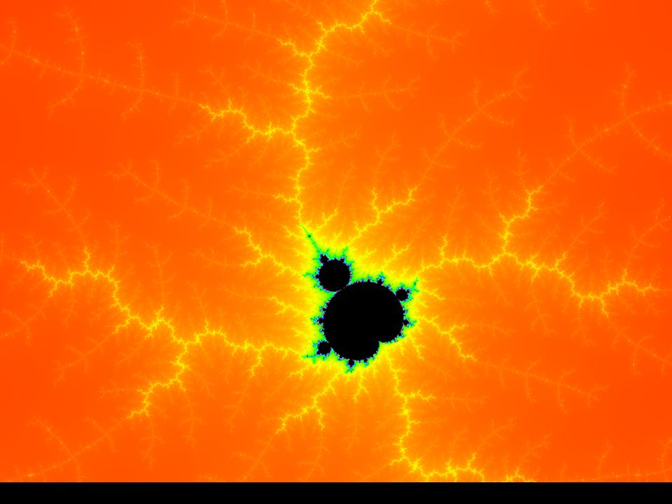
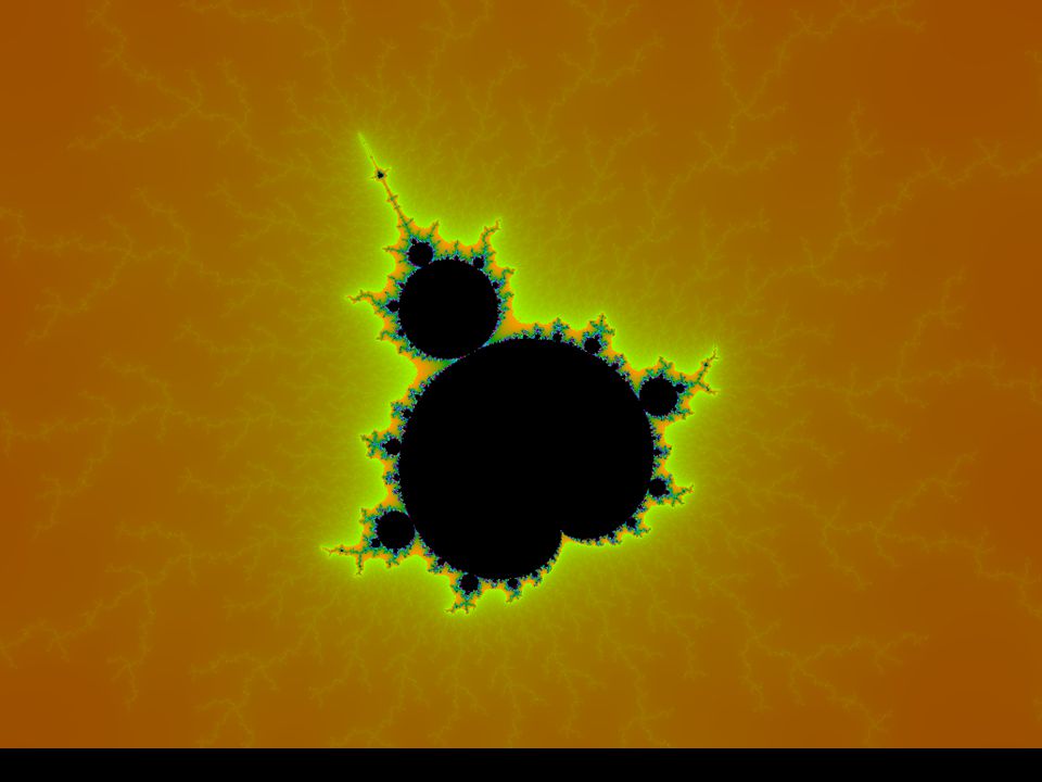
67. The Mandelbrot Set
This set has a very intricate geometry and there is a connection between the position on the Mandelbrot set and the shape of the Julia set, as well as the fate of the orbit of 0.

68. The Mandelbrot Set

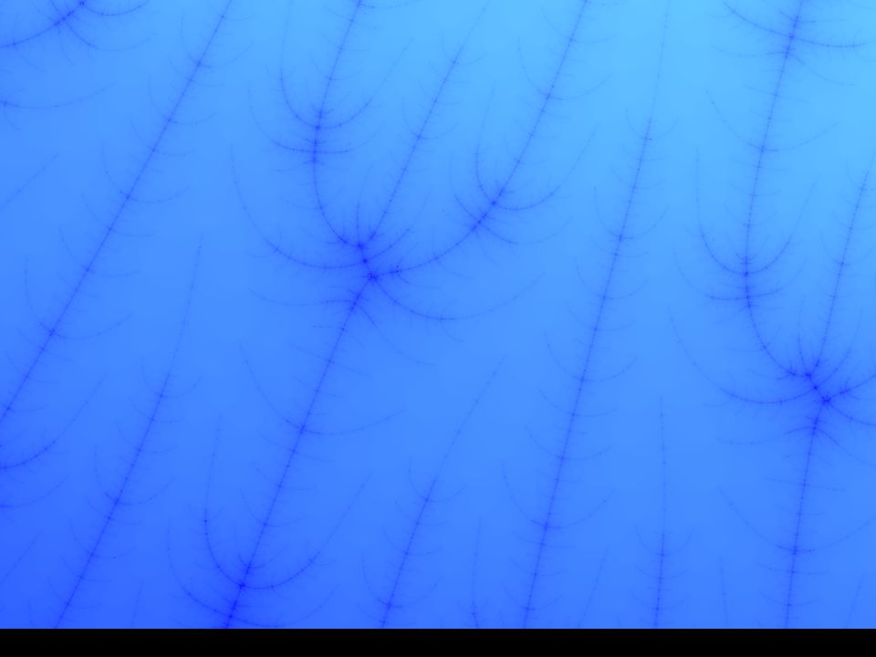
69. The Mandelbrot Set
Rather than studying the Mandelbrot set itself, quite often the region very near to the set is studied.
Here, the orbit of 0 escapes to infinity. Sometimes, though, these orbits escape slowly. The number of iterations needed for the orbit to surpass some value is counted and a color is assigned to the point based on that value. The results can be quite aesthetically pleasing.

70. There are many places where there is region almost identical to the main body of the Mandelbrot set. It can be shown that these are all connected to the main body.
Points that have the same color take the same number of iterations to surpass a predetermined value.

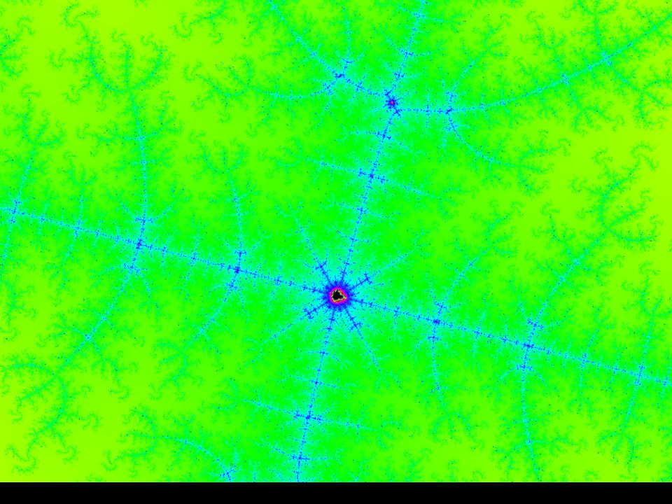
71. By changing the way the colors are assigned, different patterns can be seen.

77. Mandelbrot lichens

79. Tubes into chaos
Most of the region exhibits chaotic behavior and there are no patterns.
These tubes can be followed in as far as you can and they will continue like this.

82. Midnight over Mandelbrot

83. The Mandelbrot Set for (cr = left; cr<=right; cr+=step) {
for (ci = top; ci<=bottom; ci+=step)
zr = zi = zro = n = 0;
while (n <= nmax && (zr * zr + zi * zi)< escape_value)
zr = zr * zr - zi * zi + cr;
zi = 2 * zi * zro + ci;
zro = zr;
n++; }
if (n == nmax + 1)
color = 0;
else
color = colors[n];
SetPixel(hdc, hcenter+cr*scale, vcenter+ci*scale, color);
The basic routine (actually, it’s C) for drawing the Mandelbrot set.

84. For more information on the Julia set and the Mandelbrot set, check out the following website.

85. References
Devaney, R. & Choate, J. (2000). Chaos: A tool kit of dynamics activities. Emeryville, CA: Key Curriculum Press.
Devaney, R. (2000). The Mandelbrot and Julia sets: A tool kit of dynamics activities. Emeryville, CA: Key Curriculum Press.
All graphics produced by Ron Koehn.