Download presentation
Presentation is loading. Please wait.

1
Dose-response analysis Tjalling Jager

2
Contents Introduction Why and how of ‘dose responses’ How to fit a curve to data points (statistics) Current practice Analysis of survival data Analysis of continuous data Critical notes Limitations of current practice Outline of alternatives
 Current practice Analysis of survival data Analysis of continuous data Critical notes Limitations of current practice Outline of alternatives")
3
Why toxicity testing? How toxic is chemical X? –RA of production or use of X –ranking chemicals (compare X to Y) –environmental quality standard of X Need measure of toxicity that is: –good indicator for (no) effects in the field –comparable between chemicals Scientific interest: –how do chemicals affect organisms? –stress organism to reveal how they work …
 –environmental quality standard of X Need measure of toxicity that is: –good indicator for (no) effects in the field –comparable between chemicals Scientific interest: –how do chemicals affect organisms. –stress organism to reveal how they work ….")
4
Toxicity is a process Dynamic interaction organism↔chemical Response to toxicant depends on –toxicant –organism –endpoint (trait) –exposure duration/pattern –…–… Practical solution: standardisation –standard test protocols of OECD, ISO, ASTM etc. –required for risk assessment –scientific studies also use these protocols

5
Standard test species (aquatic) Green algae, diatoms, cyanobacteria population growth Daphnia sp. (magna) immobility reproduction ‘Well-documented’ species mortality growth life cycle
 immobility reproduction ‘Well-documented’ species mortality growth life cycle.")
6
Daphnia reproduction test 50-100 ml of well- defined test medium, 18-22°C

7
Daphnia reproduction test Daphnia magna Straus, <24 h old

8
Daphnia reproduction test Daphnia magna Straus, <24 h old

9
Daphnia reproduction test wait for 21 days, and count total offspring …

10
Daphnia reproduction test at least 5 test concentrations in geometric series …

11
Response vs. dose Response log concentration

12
Contr. Response vs. dose NOEC Response log concentration LOEC * 1. Statistical testing

13
What’s wrong? Inefficient use of data –most data points are ignored –NOEC has to be one of the test concentrations Awkward use of statistics –absence of proof is no proof of absence … –level of effect at NOEC regularly >20% –poor testing leads to high (unprotective) NOECs But, NOEC is still used …
 NOECs But, NOEC is still used ….")
14
Response vs. dose EC50 Response log concentration 1. Statistical testing 2. Curve fitting What curve to use?

15
Linear? Response log concentration

16
Threshold, linear? Response log concentration

17
Threshold, curve? Response log concentration

18
S-shape? Response log concentration

19
Hormesis? Response log concentration

20
Which curve? Popular: S-shaped curves Usually inverse cumulative probability distributions –continuous, monotonic … –e.g., log-normal, log-logistic, Weibull probability density log concentration cumulative density log concentration 1

21
Which curve? Popular: S-shaped curves Usually inverse cumulative probability distributions –continuous, monotonic … –e.g., log-normal, log-logistic, Weibull probability density log concentration cumulative density log concentration 1 1-

22
Summary of why and how Aim: quantify/summarise ‘the toxicity’ of a chemical Toxicity tests are highly standardised Classic ways to extract summary statistic: –hypothesis testing (e.g., NOEC) –curve fitting (e.g., EC50) S-shaped curves dominate –choice is quite arbitrary
 –curve fitting (e.g., EC50) S-shaped curves dominate –choice is quite arbitrary")
23
Introduction 2 How to fit a curve to data

24
optim. method Problem How to find ‘best’ parameter values? How certain are we of those? dose-resp. model data parameters predicted effect ‘error’ model

25
Example: growth Springtail Folsomia candida –cohort followed over time –weight at t=0 destructive Time (days)Weight (µg) 01.8* 1673.0 23165 30226 37242 44250 51263
Weight (µg) 01.8*")
26
Make a plot 0102030405060 -50 0 50 100 150 200 250 300 350 Time (days) Body weight (µg)
 Body weight (µg)")
27
Add a model Von Bertalanffy model for body weight –find ‘best’ values for parameters W m and r b 0102030405060 -50 0 50 100 150 200 250 300 350 Time (days) Body weight (µg)
 Body weight (µg)")
28
Residuals Can model go through all points exactly? –generally not Why not? –measurement error –biological variation –the model is always ‘wrong’ That’s true, but let’s assume... –model is completely right –data points are independent samples –error is normally distributed –same variation for all points (homoscedasticity) error model → least squares
 error model → least squares.")
29
Model fitting Minimise the squared residuals –model for weight, fix W 0 0102030405060 -50 0 50 100 150 200 250 300 350 Time (days) Body weight (µg)
 Body weight (µg)")
30
Many packages provide standard error of estimate (s.e.) Confidence: best value ±1.96 s.e. (or use t-distribution) –assumes sampling distribution of parameter is normal (or Stud.-t) Optimise 0102030405060 -50 0 50 100 150 200 250 300 350 Time (days) Body weight (µg) W m = 294 µg (241 - 347) r B = 0.0690 day -1 (0.0498 - 0.0881)
 –assumes sampling distribution of parameter is normal (or Stud.-t) Optimise Time (days) Body weight (µg) W m = 294 µg ( ) r B = day -1 ( ).")
31
Intervals on the curve Reliability of the model curve (confidence interval) Where to expect new observations (prediction interval) 0102030405060 -50 0 50 100 150 200 250 300 350 Time (days) Body weight (µg)
 Where to expect new observations (prediction interval) Time (days) Body weight (µg)")
32
Remarks … Parameter estimates and intervals follow from assumptions (the ‘error model’): –model is correct –in this case: W 0 is known –x-values are known (controlled) –errors in y are normal –errors in y are independent –errors in y constant variance –many data points (asymptotic)
: –model is correct –in this case: W 0 is known –x-values are known (controlled) –errors in y are normal –errors in y are independent –errors in y constant variance –many data points (asymptotic)")
33
Summary curve fitting What do you need? Data set and a model for the process (curve) ‘Error model’ for the deviations –normal, independent, homogeneous variances: leads to least squares –not normal, and/or not homogenous variances: transform (log-transforming is popular) use different error model (see: likelihood) Results are meaningful only when both process and error model are meaningful
 ‘Error model’ for the deviations –normal, independent, homogeneous variances: leads to least squares –not normal, and/or not homogenous variances: transform (log-transforming is popular) use different error model (see: likelihood) Results are meaningful only when both process and error model are meaningful.")
34
Current practice 1 Analysis of survival data

35
Type of endpoints Mortality/Immobility = Quantal count number of animals responding Growth/Reproduction = Graded measure degree of response for each individual –e.g., 85 eggs or body weight of 23.2 mg –between 0 and infinite –e.g., EC50 (conc. at which the mean response is 50%) –e.g., 8 out of 20 (is 40%) –always whole number (or 0-100%) –e.g., LC50 (conc. at which 50% of population is dead)
 –e.g., 8 out of 20 (is 40%) –always whole number (or 0-100%) –e.g., LC50 (conc. at which 50% of population is dead).")
36
Survival analysis Typical data set –number of live (mobile) animals: quantal data –example: Daphnia exposed to nonylphenol mg/L0 h24 h48 h 0.00420 0.03220 0.05620 0.10020 0.18020 16 0.32020132 0.5602020
 animals: quantal data –example: Daphnia exposed to nonylphenol mg/L0 h24 h48 h")
37
Plot dose-response curve Procedure –plot percentage survival after 48 h –concentration on log scale Objective –derive LC50

38
What model? Requirements curve –start at 100% and monotonically decreasing to zero –inverse cumulative distribution? –choose log-normal

39
Graphical method Probit transformation 2 3 4 5 6 7 8 9 probits std. normal distribution + 5 Linear regression on probits versus log concentration 0 20 40 60 80 100 0.0010.010.11 concentration (mg/L) 0 20 40 60 80 100 0.0010.010.11 data mortality (%)
 data mortality (%).")
40
Fit model, least squares? 0 20 40 60 80 100 0.0010.010.11 concentration (mg/L) survival (%)
 survival (%)")
41
Fit model, ‘likelihood’ mg/L0 h48 h pipi 0.00420 ≈1 0.03220 ≈1 0.05620 ≈1 0.10020 ≈1 0.1802016≈0.8 0.320202≈0.1 0.560200≈0

42
Fit model, ‘likelihood’ mg/L0 h48 h pipi 0.00420 ≈1 0.03220 ≈1 0.05620 ≈1 0.10020 ≈1 0.1802016≈0.8 0.320202≈0.1 0.560200≈0 p c b a Find a and b such that probability of data is maximised

43
Which model curve? Popular distributions –log-normal (‘probit’) –log-logistic (‘logit’) –Weibull
 –log-logistic (‘logit’) –Weibull")
44
Which model curve? 10 0 0.1 0.2 0.3 0.4 0.5 0.6 0.7 0.8 0.9 1 concentration fraction surviving data log-logistic log-normal Weibull gamma LC50log lik. Log-logistic0.225-16.681 Log-normal0.226-16.541 Weibull0.242-16.876 Gamma0.230-16.582

45
Non-parametric analysis Spearman-Kärber: wted. average of midpoints 0 20 40 60 80 100 0.0010.010.11 log concentration (mg/L) survival (%) weights: number of deaths in interval for symmetric distribution (on log scale) weights: number of deaths in interval for symmetric distribution (on log scale)
 survival (%) weights: number of deaths in interval for symmetric distribution (on log scale) weights: number of deaths in interval for symmetric distribution (on log scale).")
46
‘Trimmed’ Spearman-Kärber 0 20 40 60 80 100 0.0010.010.11 log concentration (mg/L) survival (%) Interpolate at 95%Interpolate at 5%
 survival (%) Interpolate at 95%Interpolate at 5%")
47
Distribution … of what? Perhaps ‘tolerance’ … let’s assume: –animal dies instantly when exposure exceeds ‘threshold’ –threshold varies between individuals probability density concentration

48
Concept of ‘tolerance’ 1 1-cumulative density 1 20% mortality

49
What is the LC50? 1 1-cumulative density 1 50% mortality ?

50
Summary: survival data Survival data are ‘quantal’ responses –data are fraction of individuals responding –one possible mechanism is ‘tolerance distribution’ Analysis types –regression (e.g., log-logistic or log-normal) LC50 or LCx –non-parametric (e.g., Spearman-Kärber) LC50 LC50 is … –estimated concentration at which 50% of the population is dead –(for specific exposure time/test conditions)
 LC50 or LCx –non-parametric (e.g., Spearman-Kärber) LC50 LC50 is … –estimated concentration at which 50% of the population is dead –(for specific exposure time/test conditions)")
51
Current practice 2 Analysis of continuous data

52
Type of endpoints Mortality/Immobility = Quantal count number of animals responding Growth/Reproduction = Graded measure degree of response for each individual –e.g., 85 eggs or body weight of 23.2 mg –between 0 and infinite –e.g., EC50 (conc. at which the mean response is 50%) –e.g., 8 out of 20 (is 40%) –always whole number (or 0-100%) –e.g., LC50 (conc. at which 50% of population is dead)
 –e.g., 8 out of 20 (is 40%) –always whole number (or 0-100%) –e.g., LC50 (conc. at which 50% of population is dead).")
53
Analysis of continuous data Endpoints for individual –in ecotoxicology, usually growth or reproduction Two approaches –hypothesis testing: NOEC/LOEC –curve fitting: EC50 or in general: ECx

54
Regression modelling Select model –log-logistic most popular –we cannot talk about a tolerance distribution! 0 5 10 15 20 110100 concentration (mg/L) survival LC50 0 20 40 60 80 100 120 00.1110 concentration (mg/L) total offspring/female EC50
 survival LC concentration (mg/L) total offspring/female EC50.")
55
Least-squares estimation concentration (mg/L) 0 20 40 60 80 100 0.0010.010.11 reproduction (#eggs)
 reproduction (#eggs)")
56
Example: Daphnia repro Plot concentration on log-scale 10 -2 10 10 0 1 0 20 30 40 50 60 70 80 90 100 concentration # juv./female

57
Example: Daphnia repro Fit sigmoid curve Estimate ECx from the curve 10 -2 10 10 0 1 0 20 30 40 50 60 70 80 90 100 concentration # juv./female EC10 0.13 mM (0.077-0.19) EC50 0.41 mM (0.33-0.49)
 EC mM ( )")
58
Summary: continuous data Repro/growth data are ‘graded’ responses –look at mean response of individual animals –not fraction of animals responding –thus, we cannot talk about ‘tolerance distribution’ Analysis types –statistical testing NOEC –regression (e.g., log-logistic) ECx –note: estimates and intervals assume …
 ECx –note: estimates and intervals assume …")
59
Critical notes Limitations of current practice

60
If EC50 is the answer … … what was the question? “What is the concentration of chemical X that leads to 50% effect on the total number of offspring of Daphnia magna (Straus) after 21-day constant exposure under standardised laboratory conditions?”
 after 21-day constant exposure under standardised laboratory conditions .")
61
Why 21 days? Toxicity is a process in time … statistics like LC50/ECx/NOEC change in time this is hidden by strict standardisation –Daphnia mortality:2 days –fish mortality:4 days –Daphnia repro21 days –fish growth28 days –…–…

62
24 hours Survival effects 00.10.20.30.40.50.60.7 0 0.1 0.2 0.3 0.4 0.5 0.6 0.7 0.8 0.9 1 concentration fraction surviving 48 hours LC50s.d. tolerance 24 hours0.3700.306 48 hours0.2260.267

63
Sub-lethal tests With time, control response increases and all parameters may change … increasing time (t = 9-21d)
")
64
EC10 in time 0.5 1 1.5 2 2.5 05101520 0 survival body length cumul. reproduction carbendazim Alda Álvarez et al. (2006) time (days) 0246810121416 0 20 40 60 80 100 120 140 pentachlorobenzene time (days)
 time (days) pentachlorobenzene time (days).")
65
Concluding on test duration Effects change in time, how depends on: –endpoint, species, chemical … –environmental conditions No such thing as the ECx –always report endpoint and test duration –is it a useful summary statistic? Watch out when … –comparing species, chemicals, endpoints … –using ECx to judge ‘safety’ of a chemical …

66
What about alternatives? Rethink the question leading to ECx … “What is the concentration of chemical X that leads to 50% effect on the total number of offspring of Daphnia magna (Straus) after 21-day constant exposure under standardised laboratory conditions?” Better questions start with “How …” or “Why …” But, biology is so complex …
 after 21-day constant exposure under standardised laboratory conditions Better questions start with How … or Why … But, biology is so complex ….")
67
Dealing with complexity Environmental chemistry … –predict the concentrations of chemicals in the environment –from emissions and physico-chemical properties

68
Make an idealisation E.g., multimedia-fate or ‘box’ models

69
external concentration (in time) toxico-kinetic model toxico-kinetic model For effects: TKTD modelling internal concentration in time process model for the organism process model for the organism effects on endpoints in time toxicokinetics toxicodynamics
 toxico-kinetic model toxico-kinetic model For effects: TKTD modelling internal concentration in time process model for the organism process model for the organism effects on endpoints in time toxicokinetics toxicodynamics")
70
More information on TKTD modelling:www.debtox.info Summercourse dynamic modelling for toxic effects, August 2018 (DK)
")
71
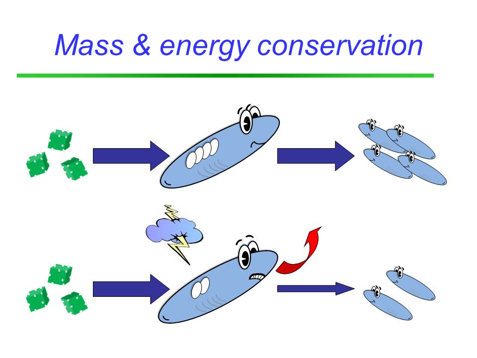
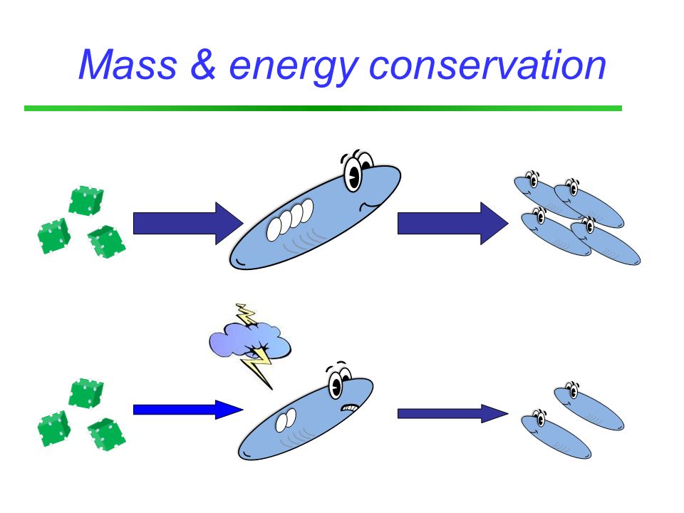
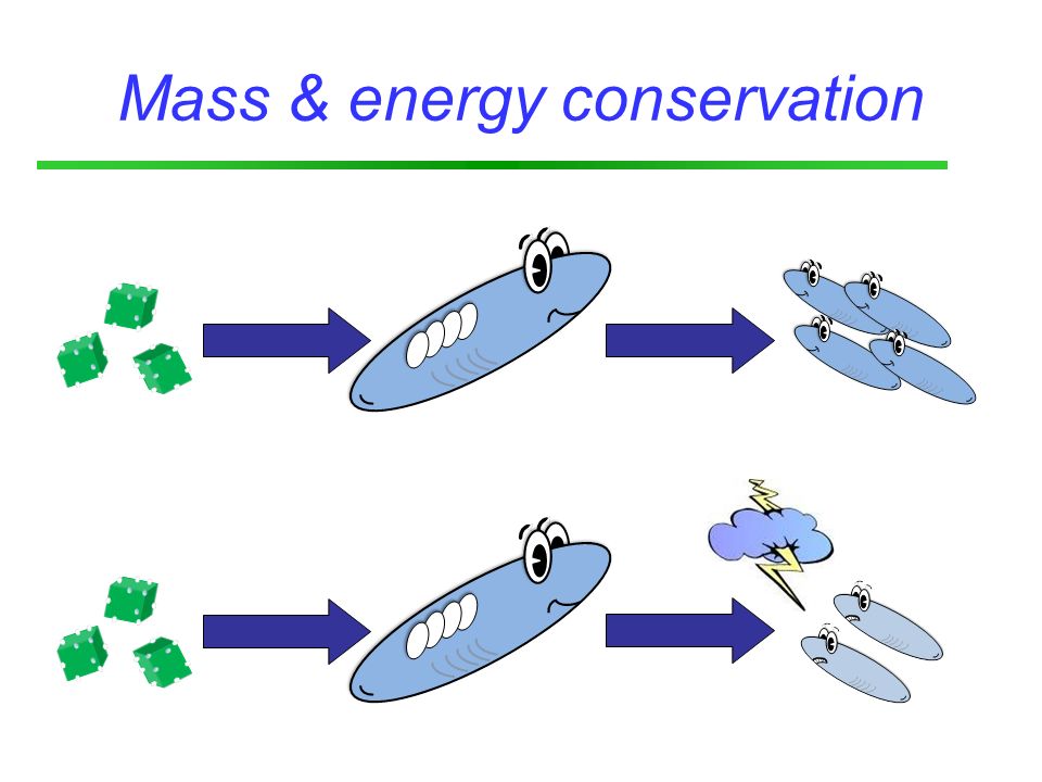
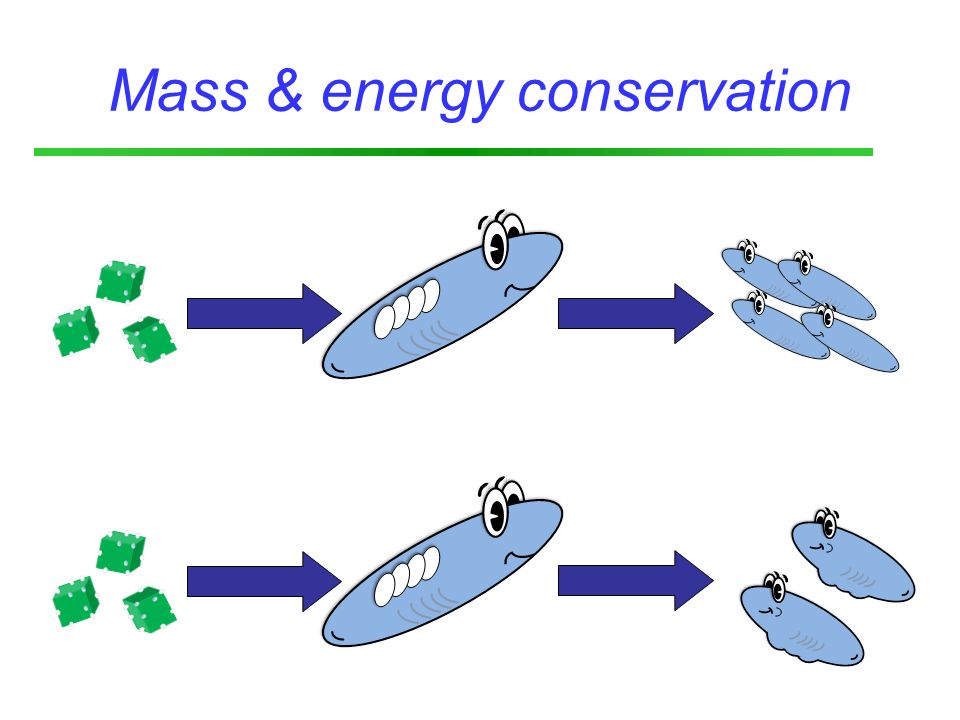
Mass & energy conservation

76
Dynamic Energy Budget Organisms obey mass and energy conservation –find the simplest set of rules... –over the entire life cycle... –for all organisms (related species follow related rules)
.")
77
growth and repro in time DEBtox basics DEB toxicokinetics Assumptions - effect depends on internal concentration - chemical changes parameter in DEB model

78
Ex.1: maintenance costs time cumulative offspring time body length TPT Jager et al. (2004)
")
79
Ex.2: growth costs time body length time cumulative offspring Pentachlorobenzene Alda Álvarez et al. (2006)
.")
80
Ex.3: egg costs time cumulative offspring time body length Chlorpyrifos Jager et al. (2007)
")
Similar presentations


>")
 stress in DEB 2: toxicokinetics Tjalling Jager Dept. Theoretical Biology TexPoint fonts used in EMF. Read the TexPoint manual before.>")


 theory by Elke, Svenja and Ben.>")

>")


 by multiple organizations American Society.>")

 stress in DEB 3: the ‘target site’ and effects on survival Tjalling Jager Dept. Theoretical Biology TexPoint fonts used in EMF. Read.>")

