1. The Normal Distribution Chapter 3

2. When Exploring Data Always start by plotting your individual variables Look for overall patterns (shape, centre, spread) and for deviations such as outliers Calculate appropriate summary statistics to identify the centre and spread

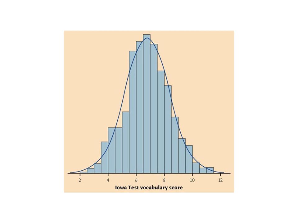
3. Density Curves and Normality Sometimes data takes on a recognizable shape Density Curves are those that: –Are always on or above the (x) axis –Have exactly an area of 1 under the curve Density curves come in all shapes and sizes and can be centred or skewed.

5. Describing a density curve Our measures of central tendency and dispersion work just as well on density curves as on actual observations Although these are theoretical constructions we can describe them like real data

6. A special set of curves Normal curves are a subset of density curves all are –Symmetrical and single peaked –It is completed described by giving its mean μ and standard deviation Ố –The mean is at the centre of the distribution and is the same as the median –Changing μ without changing Ố moves the graph but does not alter it –The larger Ố is the more spread out the curve is.

7. The Normal Curve and the 68-95-99.7 rule

8. The abbreviation of a Normal Distribution In the rest of the book the parameters of a normal distribution are summarized by the notation

9. Why is the normal dist. so important? It is a good description of the distribution of some important real world data It is a good approximation of many chance outcomes Statistical tests with distributions based on normality work just as well with many non- normal but roughly symmetrical distributions. In many statistical inference procedures there is an assumption of normality we test against. If the results we see could be expected to occur, then there is little reason to believe we have found a meaningful result

10. This is handy One reason normality is handy is because it provides us a way to standardize variables so that we can in fact compare apples and oranges (or at least variables measured on two different scales). Suppose you are interested in how educating girls (measured in average years enrolled in schooling) and international trade (measured in dollars) impact economic development How can you clearly state the impact of years of schooling and dollars in the same equation?

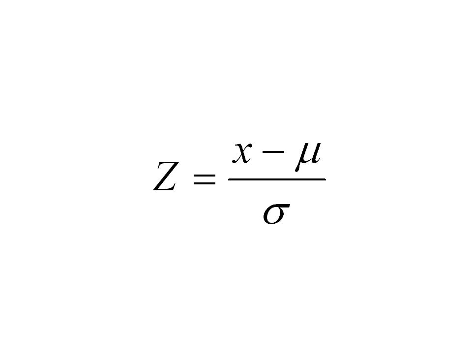
11. What you can do is convert each set of scores so that each observation is expressed as a measure of how far it falls away (either positively or negatively) from the mean for the variable in question.

13. As a result the two variables will now be on a common scale and you can compare the impact of schooling for girls and international trade on economic development.

14. Finally, as the example in the book shows If you believe your observations are normally distributed and you know the Mean and Standard Deviation, you can work out proportions In the case they show in the book the question was what proportion of first year university students were likely to be eligible to play sports, given the league requirement that they score 820 on the SAT before beginning their first year of university.

15. If we know the total area under a normal curve is = 1 and we subtract the area to the left of 820 we will have an answer. To work out the area you need to: guess, use a calculator or software or the applet on the book website, or convert the information to Z scores and use Table A.

16. Guestimation Distribution is normal; Mean = 1026; Std.D.= 209. Therefore the value = 1 st Std. below mean is 817 which is pretty close to 820 (the score you need so as to be eligible) Therefore we have 68% + the rest of the right side = 68 + (100-68)/2 = 68 + 16 = 84% Approximately 84% of students qualify

17. Using software or the applet To do the applet we will go to the website for the book http://bcs.whfreeman.com/bps5e/

18. Using Excel as a software example To use Excel you would go to the stats plugin and select Probability Calculations Normal Distribution

19. Using the Z scores and tables Start by calculating the Z score that would correspond to a score of 820 Therefore we need to find the area under the normal curve which is equal to -0.99

20. To use the table you first find the row that corresponds to the first digit -0.9 then draw your finger across until you find the column for the second in this case “.09) Therefore the answer is.1611

21. So now that we have found the area under the normal curve when expressed as Z scores that corresponds to a score of 820 it is the same mathematical problem as before 1 – 0.1611≈ 84% Therefore about 84% of students would qualify to play sports

22. Have a fun week Nikolai Bogdanov-Belsky Counting in their heads (1895) Posted on line by Tamir Khason Khason.net