4. Trajectory Data: Analysis and Patterns Pattern Recognition 2015/2016

5. Algorithms Operate on Data Tasks (scheduling) Graphs (path planning, flow) Numbers for math problems (prime testing, partition) Linear inequalities (optimization) Time series (data mining: trends, outliers)

6. Trajectories Model for the movement of a (point) object; the model: f : [ time interval ]  2D or 3D

7. Trajectories Model for the movement of a (point) object; the model: f : [ time interval ]  2D or 3D The path of a trajectory is just any curve

8. Trajectories Model for the movement of a (point) object Many useful applications in different disciplines (including the real World)

9. Tracking Vehicles

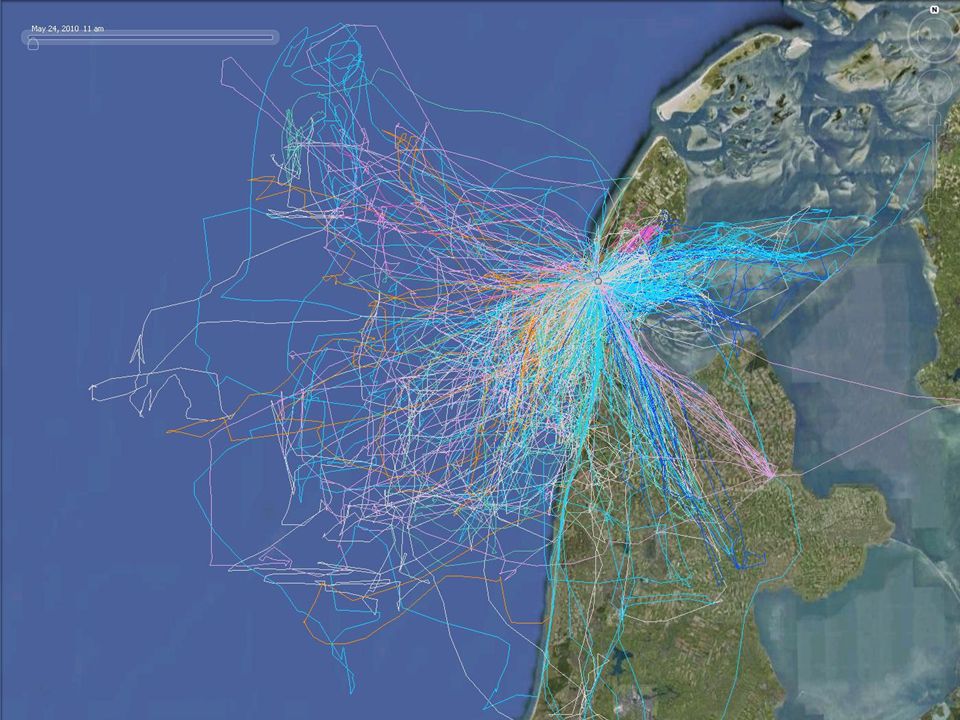
10. Tracking Animals

11. Tracked Turtle

12. Tracking Insects

13. Tracking People

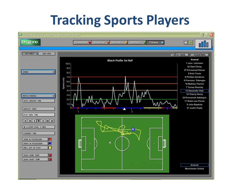
14. Tracking Sports Players

16. Tracking Hurricanes

17. Tracking Technology GPS, RFID, video analysis, … – Range – Precision – Sampling rate

18. Tracking Technology GPS – Range – Precision – Sampling rate

19. Tracking Technology GPS – Range: whole world – Precision: 2-10 meters in lat-lon, worse in elevation Suffers from urban canyons, tree cover, clouds, … – Sampling rate: depends on device, energy source, need not be regular

20. Trajectory Data The data as it is acquired by GPS: sequence of triples (spatial plus time-stamp); quadruples for trajectories in 3D (x i,y i,t i ) (x 2,y 2,t 2 ) (x 1,y 1,t 1 ) (x n,y n,t n )

21. Trajectory Data Typical assumption for sufficiently densely sampled data: constant velocity between consecutive samples  velocity/speed is a piecewise constant function (x i,y i,t i ) (x 2,y 2,t 2 ) (x 1,y 1,t 1 ) (x n,y n,t n )

22. Trajectory Data Analysis Address practical questions like: “How much time does a gull typically spend foraging on a trip from the colony and back?”

23. Trajectory Data Analysis Address practical questions like: “How much time does a gull typically spend foraging on a trip from the colony and back?” “If customers look at book display X, do they more often than average also go to and look at bookshelf Y?”

24. Trajectory Data Analysis Address practical questions like: “How much time does a gull typically spend foraging on a trip from the colony and back?” “If customers look at book display X, do they more often than average also go to and look at bookshelf Y?” “How and where is the change of direction in a starling flock initiated?”

25. Trajectory Data Analysis Abstract/general purpose questions: Single trajectory – simplification, cleaning – segmentation into semantically meaningful parts – finding recurring patterns (repeated subtrajectories) Two trajectories – similarity computation – subtrajectory similarity Multiple trajectories – clustering, outliers – flocking/grouping pattern detection – finding a typical trajectory or computing a mean/median trajectory – visualization

27. Trajectory Analysis Research discussed here: – Segmentation of trajectories – Subtrajectory similarity – Trajectory grouping structure

28. Segmentation Cutting a trajectory in pieces that are “similar” within the piece

29. Segmentation Cutting a trajectory in pieces that are “similar” within the piece

30. Segmentation in other Areas Image segmentation: partition a digital image in parts with similar characteristics (hopefully meaningful pieces)

31. Segmentation in other Areas Time-series segmentation: partition time series data into pieces with similar characteristics

32. Segmentation Cutting a trajectory in pieces that are “similar” within the piece

33. Why Segmentation? Explaining behavior of a moving entity: one type of behavior may be characterized by similarity of movement  semantic annotation Detecting outliers: short segments in a segmentation may be caused by outliers

34. Why Segmentation? Explaining behavior of a moving entity: one type of behavior may be characterized by similarity of movement  semantic annotation Dagstuhl seminar: Representation, Analysis, and Visualization of Moving Objects (2010); break-out group : Gull data (Emiel van Loon, Jörg-Rüdiger Sack, Kevin Buchin, Maike Buchin, Mark de Berg, MvK, Joachim Gudmundsson, David Mountain)

35. Segmentation Cutting a trajectory in pieces that are “similar” within the piece “Similar” can refer to heading, speed, curvature, sinuosity, … We want few pieces (no over-segmentation) How do we define “similar”?

36. Segmentation: heading On every edge of the trajectory, heading is well-defined Similarity can mean: in the same cardinal direction Northbound EastWest South

37. Segmentation: heading On every edge of the trajectory, heading is well-defined Similarity can mean: in the same cardinal direction Northbound EastWest South eastbound northbound westbound southbound

38. Segmentation: heading On every edge of the trajectory, heading is well-defined Similarity can mean: in the same cardinal direction Northbound EastWest South

39. Segmentation: heading On every edge of the trajectory, heading is well-defined Similarity can mean: in the same cardinal direction Northbound EastWest South We would segment at every vertex, while we want one single segment bad idea

40. Segmentation: heading Use relative directions: We require that within any single segment the headings are within an angle  /2 everywhere

41. Segmentation: heading Use relative directions: We require that within any single segment the headings are within an angle  /2 everywhere

42. Segmentation: heading Use relative directions: We require that within any single segment the headings are within an angle  /2 everywhere

43. Segmentation: heading Use relative directions: We require that within any single segment the headings are within an angle  /2 everywhere

44. Segmentation: heading Use relative directions: We require that within any single segment the headings are within an angle  /2 everywhere

45. Segmentation: speed Linear interpolation of position between the vertices makes speed piecewise constant (constant on every edge) Segmentation can be based on absolute intervals like [0-2], [2-5], [5-10], [10-15], [15-20], [20-30], [30-..] km/h 3129312931293129

46. Segmentation: speed Linear interpolation of position between the vertices makes speed piecewise constant (constant on every edge) Segmentation can be based on absolute intervals like [0-2], [2-5], [5-10], [10-15], [15-20], [20-30], [30-..] km/h Segmentation can also be based on relative speeds: within any single segment the speed ratio is at most, say, 1.5 (alternatively: the speed difference is at most 10 km/h)

47. Segmentation: conjunction Suppose we require that within any single segment: – the headings are within an angle  /2 everywhere, and – the speed ratio is at most 2

48. Segmentation: heading and speed Suppose we require that within any single segment: – the headings are within an angle  /2 everywhere, and – the speed ratio is at most 2 speed heading

49. Segmentation: heading and speed Combining the optimal segmentations on heading and on speed is not optimal for the combined criterion speed heading

50. Segmentation In all three cases (heading, speed, heading&speed), a greedy approach works: make each next segment as long as possible Trivial from the algorithms perspective: O( n ) time for a trajectory with n vertices need to compare with and update the extreme headings (or speeds)

51. Segmentation: location Segmentation on location: segment must fit inside some (well-placed) circle of a given radius, also greedy Segmentation may happen between vertices Less easy from the algorithmic perspective: O( n log n ) time for a trajectory with n vertices (involves an LP-type problem)

52. Segmentation: attributes Heading, speed and location are examples of attributes that are defined at (almost) every point on the trajectory There are more criteria, like curvature, sinuosity, and curviness  need a framework to handle different criteria and different ways of combining them

53. Segmentation: framework Attribute: some value defined at every point on the trajectory (location, heading, speed, curvature, …) Criterion: restriction on allowed values of an attribute within the same segment (speed ratio at most 2, change of heading at most 3, etc.) Segmentation on any combination (conjunction or disjunction) of criteria

54. Segmentation: framework Attributes Criteria Segmentation on any combination:  Criteria satisfied within each segment  Optimal (minimum number of segments)

55. Segmentation: monotonicity Definition: A criterion is monotone if satisfaction for a segment implies satisfaction for any subsegment Absolute or relative heading is monotone Absolute or relative speed is monotone Location by enclosing circle or by diameter is monotone Curvature criteria are monotone Curviness, sinuosity also  implies 

56. Segmentation: monotonicity Definition: A criterion is monotone if satisfaction for a segment implies satisfaction for any subsegment Theorem: For any monotone criteria, if a subtrajectory with m vertices can be tested in O(T( m )) time and the furthest point satisfying the criteria on a given edge can be found in O(F( m )) time, then optimal segmentation takes O(T( n ) log n + F( n )) time For the given criteria: optimal segmentation in O( n ) or O( n log n ) time

57. Segmentation: Algorithm

58. Migrating geese Alewijnse, Buchin, Buchin, Kölzsch, Kruckenberg, Westenberg (2014)

59. Migrating geese Alewijnse, Buchin, Buchin, Kölzsch, Kruckenberg, Westenberg (2014)

60. How about non-monotone criteria?

61. Non-monotone Segmentation Non-monotone criteria: – standard deviation (of e.g. speed) below a threshold – at most 5% of the time outlying speed (not within factor 1.5) 2 m/s 5 m/s 3 m/s standard deviation  1 m/s

62. Non-monotone Segmentation Non-monotone criteria: – standard deviation (of e.g. speed) below a threshold – at most 5% of the time outlying speed (not within factor 1.5) start stop a b a b possible segments (time intervals) (time)

63. Non-monotone Segmentation Non-monotone criteria: – standard deviation (of e.g. speed) below a threshold – at most 5% of the time outlying speed (not within factor 1.5) start stop segmentation

64. Non-monotone Segmentation Non-monotone criteria: – standard deviation (of e.g. speed) below a threshold – at most 5% of the time outlying speed (not within factor 1.5) start stop forbidden segments

65. Non-monotone Segmentation Non-monotone criteria: – standard deviation (of e.g. speed) below a threshold – at most 5% of the time outlying speed (not within factor 1.5) start stop forbidden segments

66. Non-monotone Segmentation Non-monotone criteria: – standard deviation (of e.g. speed) below a threshold – at most 5% of the time outlying speed (not within factor 1.5) start stop forbidden segments for monotone criteria

67. Non-monotone Segmentation Abstract minimum staircases, any forbidden regions with n edges  NP-hard

68. Non-monotone Segmentation When forbidden regions come from our non-monotone criteria on trajectories, the minimum staircase problem can be solved in polynomial time start stop

69. Non-monotone Segmentation When forbidden regions come from our non-monotone criteria on trajectories, the minimum staircase problem can be solved in polynomial time start stop

70. Non-monotone Segmentation For the outlier criterion, the forbidden region in a single cell is always the common intersection of at most four half-planes

71. Non-monotone Segmentation Compute the forbidden region in each of the O( n 2 ) cells of the start-stop diagram Starting at k = 1, compute what can be reached in k steps using what can be reached in k – 1 steps and increment k When we reach the end of the trajectory, finish

72. Non-monotone Segmentation Non-monotone criteria: – standard deviation (of e.g. speed) below a threshold – at most 5% of the time outlying speed Segmentation on these criteria takes O( k n 2 ) or O( k n 2 log n ) time, where k is the optimal number of segments For certain non-monotone criteria, no efficient algorithm seems to exist (e.g. conjunctions)

73. Topic 2: subtrajectory similarity

74. Similarity of trajectories Inverse of “distance” Important for clustering Various measures possible

75. Similarity of trajectories Inverse of “distance” Important for clustering Various measures possible Hausdorff: maximum of some point on one trajectory to nearest point on other trajectory

76. Similarity of trajectories Inverse of “distance” Important for clustering Various measures possible Frechet: minimum leash length for a child and dog to traverse the whole trajectory, without going back (child nor dog)

77. Hausdorff distance and Frechet distance are measures for shapes, not for trajectories

78. Similarity of trajectories Inverse of “distance” Important for clustering Various measures possible Time-aware: maximum distance for pairs of points at the same time

79. Similarity of trajectories Inverse of “distance” Important for clustering Various measures possible Average time-aware: average distance over all pairs of points at the same time

80. Why sub-trajectory similarity? The start behavior of an entity/trajectory may be a-typical (animal just after giving it a radio collar) The start of a phenomenon may be gradual (hurricane builds up in force)

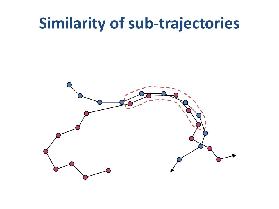
81. Similarity of sub-trajectories

83. Average time-aware distance  1 (t) is the position of entity 1 at time t  2 (t + t shift ) is the position of entity 2 at time t + t shift t s is the start time; T is the duration

84. Subtrajectory similarity Simplest version: same starting times of subtrajectory (but unknown), duration T given, can be solved in linear time Idea: increase t s to perform a scan over the trajectories minimize with fixed T

85. Subtrajectory similarity The problem becomes: Find t s such that the area below the graph from t s to t s +T is minimum Between two endpoints, the graph is a hyperbolic function tsts t d(  1 (t),  2 (t)) t s +T

86. Subtrajectory similarity Updating the area function (expressed in t s ) below the graph when t s to t s + T passes an endpoint can be done in O(1) time, optimizing the function too The scan takes O(n) time in total tsts t d(  1 (t),  2 (t)) t s +T

87. Trajectory similarity and clustering With a similarity measure for trajectories, certain clustering methods are directly applicable: – single linkage clustering – complete linkage clustering – (if we can identify a representative) k-medoids clustering – (if we can identify a mean) k-means clustering For single linkage and complete linkage clustering, compute a matrix with all (n choose 2) similarity measures Start with singleton clusters and merge the “closest two” iteratively, until k clusters remain

88. Topic 3: grouping structure

89. Grouping Structure How does one define and compute the ensemble of moving entities forming groups, merging with other groups, splitting into subgroups? … define and compute …  formalization + algorithms

90. Previous Work Flocks [Gudmundsson, Laube, Wolle, Speckmann, …. (2005- )] Herds [Huang, Chen, Dong (2008)] Convoys [Jeung, Yiu, Zhou, Jensen, Shen (2008); Aung, Tan (2010)] Swarms [Li, Ding, Han, Kays (2010)] Moving groups/clusters [Kalnis, Mamoulis, Bakiras (2005); Wang, Lim, Hwang (2008); Li, Ding, Han, Kays (2010)] t=1t=3 t=5t=7 t=2 t=4t=6 t=8

91. The Results Use whole trajectory (interpolated) instead of discrete time stamps only (as opposed to herds, swarms, convoys, …) Study the whole grouping structure with merging, splitting, … (as opposed to finding flocks) Use a mathematically clean model Complexity and efficiency analysis Implementation and testing for plausibility t=1t=3 t=5t=7 t=2 t=4t=6 t=8

92. Grouping

94. Three criteria for a group: – big enough (size m) – close enough (inter-distance d) – long enough (duration δ) Only maximal groups are relevant Otherwise, assuming m=4, if 8 entities form a group during δ (or longer), then also all 162 subgroups of size at least 4 during that same time interval (maximal in group size, starting time or ending time)

95. Grouping Trace the connected components of moving disks whose radius is half the specified inter-distance, d/2

96. 0 1458 10 time Grouping Trace the connected components of moving disks whose radius is half the specified inter-distance, d/2

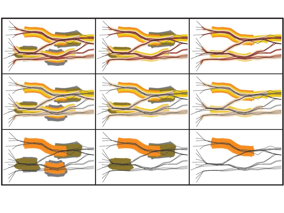
97. Grouping Maximal groups (m=2, δ =3): – { green, blue }: [0-4] – { green, blue, red }: [1-4] – { blue, red}: [1-5] – { green, purple }: [8-10] Maximal groups (m=3, δ =3): – { green, blue, red }: [1-4] Maximal groups (m=2, δ =4): – { green, blue }: [0-4] – { blue, red}: [1-5]

98. minimum group size 3 For illustration: x-coordinate is time

100. Grouping Structure Reeb graph (from computational topology): structure that captures the changes in connectivity of a process, using a graph – Edges are connected components – Vertices are changes in connected components (events) From 1 to 2 connected components

101. Grouping Structure Reeb graph; disregard group size (m = 1) and duration (δ = 0)

102. Grouping Structure Reeb graph; disregard group size (m = 1) and duration (δ = 0) purple red, blue, green blue, green red green purple, green red blue red, blue t=0 t=1t=4 t=5 t=8 t=10 t=0 t=10 edges ~ connected components vertices ~ events (changes in connected components)

103. Computing the Grouping Structure Assume t time steps and n entities Assume piecewise-linear trajectories and constant speed on pieces The Reeb graph has O( t n 2 ) vertices and edges; this bound is tight in the worst case Its computation takes O( t n 2 log n ) time

104. Computing the Maximal Groups Given a value for group size m and duration δ and distance: Compute the Reeb graph using distance d Annotate its edges and vertices Process the vertices in time-order, maintaining known maximal groups Filter the maximal groups (using m and δ) purple red, blue, green blue, green red green purple, green red blue red, blue t=0 t=1t=4 t=5 t=8 t=10 t=0 t=10

105. Computing the Maximal Groups Given a value for group size m and duration δ and distance: Compute the Reeb graph using distance d Annotate its edges and vertices Process the vertices in time-order, maintaining known maximal groups Filter the maximal groups (using m and δ) No existing maximal group ends, the maximal groups of the two branches are joined and maintained with the new branch One new maximal group starts and is maintained merge

106. Computing the Maximal Groups Given a value for group size m and duration δ and distance: Compute the Reeb graph using distance d Annotate its edges and vertices Process the vertices in time-order, maintaining known maximal groups Filter the maximal groups (using m and δ) Any existing maximal group with at least one of each new component ends and is reported New maximal groups can start on both branches; they are maintained split

107. Computing the Maximal Groups Processing a vertex takes linear time  computing all maximal groups costs O( t n 3 ) time (plus output size) There are at most O( t n 3 ) maximal groups, this bound is tight in the worst case

108. The Grouping Structure A simple, clean model for grouping / moving flocks / … Proofs of desirable properties Algorithms for the computation of the grouping structure and the maximal groups, with efficiency bounds Adaptations to get robust grouping Plausible, based on implementation

109. Grouping in Environments Extension: if distance should not be measured in a straight line, but geodesic amidst obstacles, what can we do? d two groups wall

110. Research Trends Algorithms for dealing with real data: filling in missing data, providing accuracy estimates, … Detecting patterns that involve interaction between moving entities Trajectory analysis incorporating other data (heart-rate, environment) Proper visualization for various applications and situations Algorithms, implementations and tests for specific, applied research questions (gap theory – application)