1. Image Segmentation and Active Contour
Drawing by some archeologist
Segment out the vase from the image
With what we have learned so far, what would (could ) you do?

2. Active Contour (aka snake, deformable contour)
Better idea: try to fit the boundary with some curve (closed contour).
Contour no longer belong to a small family such as ellipse or circles. The shape conforms to the object boundary.

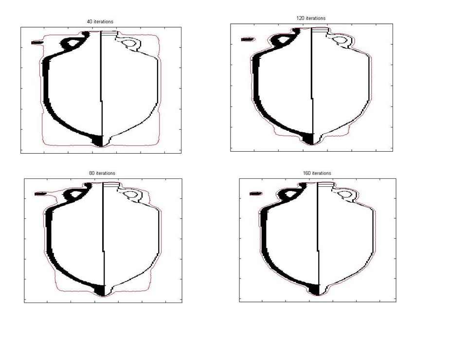
3. Vase

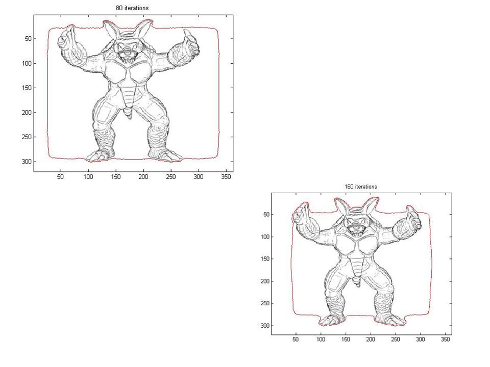
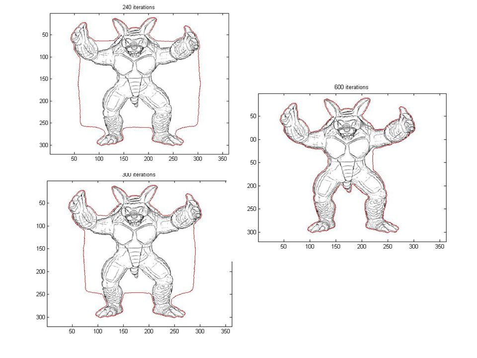
5. Armadillo

8. Details How to represent contours? Explicit scheme Implicit scheme
How to characterize the desired contour
As the (global) minimum of the a cost function.
How to deform the contour?
Discrete optimization (typically for explicit scheme)
Partial differential equation (for implicit scheme).

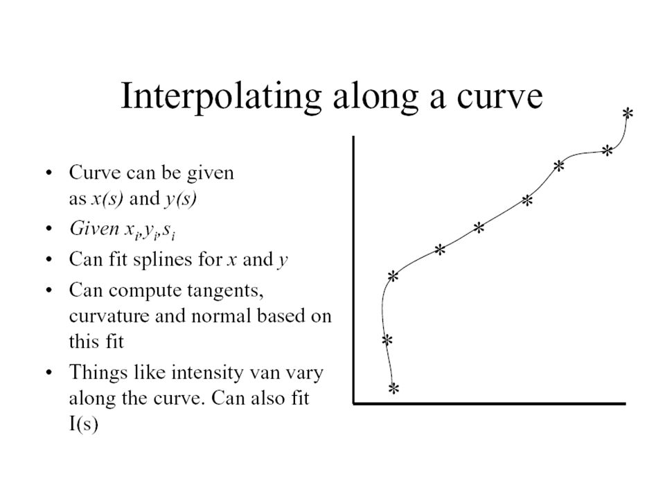
9. Contour Representation (explicit scheme)
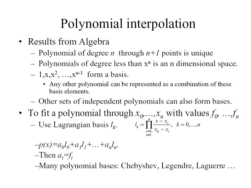
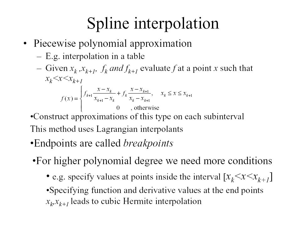
A contour is represented as
A collection of control points
An interpolating scheme
Linear interpolation gives a piecewise linear curve
Other interpolation scheme such as splines give smoother curve.
MATLAB has several routines on splines and polynomial interpolations.

13. Contour Representation (implicit scheme)
Represent a contour as the zero levelset of a continuous function. No need to keep track of the control points.
Given a contour, one such continuous function is the signed distance function from the contour.
The value at each point is the distance to the given contour. Exterior points are assigned positive values and interior points have negative values. + -

14. What is the desired contour?
Variational framework: Express the desired contour as the minimum of a energy functional (cost function).
s is the arc-length parameterization of the contour C=C(s).
Each term in the energy functional correspond to forces acting on the contour.
control the relative strength of the corresponding energy term and they vary along the contour.

15. The first two terms, continuous and smoothness constraints, are internal to the contour. The third term, an external force, accounts for the edge attraction, dragging the contour toward the closest image edge.
(minimizes contour length)
in discrete form
or better to prevent clusters

16. The second term minimizes the curvature to avoid zigzags or oscillations.
Curvature is related to the second derivatives and using central difference, the second derivatives can be approximated by
What is curvature? Curvature measures how fast the tangents of the contour vary.

17. More on curvature
is the tangent angle
If (x, y) gives the parameterization

18. Edge Attraction term
This terms depend only on the contour and independent of its derivatives.
In general, are set to constants and their values will influence the result.

19. Deforming the contour
Staring from a collection of points, find the contour which fits the target image contour best, by minimizing the energy functional
Move each control point iteratively.

20. Deforming Contour Greedy minimization Corner Elimination
Find point in a small neighborhood that minimizes the energy functional
Small neighborhood means low computational load
Corner Elimination
Search for corners as curvature maxima along the contour. Set bi = 0 for points with maximal curvature. Neglecting contribution from these points keep the contour piecewise smooth.

21. Inputs: Image I and a chain of points on the image
Algorithm Snake
Inputs: Image I and a chain of points on the image
f the minimum fraction of snake points that must move in each iteration and U(p) a small neighborhood of p and d (the average distance).
For each i= 1, .. , N, find the location in U(pi) for which the energy functional is minimum and move the control point pi to that point.
For each i=1, …, N, estimate the curvature and look for local maxima.
Set bi= 0 for all pi at which the curvature has a local maximum or exceeds some user-defined value.
Update the value of the average distance, d.

22. Main problem with explicit scheme
Keeping track of control points make can be cumbersome. In particular, topological change is difficult to execute correctly.

23. Implicit Scheme is considerably better with topological change.
Transition from Active Contours:
contour v(t)  front (t)
contour energy  forces FA FC
image energy  speed function kI
Level set:
The level set c0 at time t of a function (x,y,t) is the set of arguments { (x,y) , (x,y,t) = c0 }
Idea: define a function (x,y,t) so that at any time,
(t) = { (x,y) , (x,y,t) = 0 }
there are many such 
 has many other level sets, more or less parallel to 
only  has a meaning for segmentation, not any other level set of 

24. Need to figure out how to evolve the level set function!

25. Level Set Framework
Usual choice for : signed distance to the front (0)
 - d(x,y, ) if (x,y) inside the front
(x,y,0) =  “ on “
 d(x,y, ) “ outside “
(x,y,t) -2 5 -1 -2 -3 1 2 3 4 7 5 6
(t)
(x,y,t)

26. Level Set (x,y,t) (x,y,t+1) = (x,y,t) + ∆(x,y,t)-1 -2 -3 1 2 3 4 7 5 6
no movement, only change of values
the front may change its topology
the front location may be between samples 1 -1 -2 -3 2 3 4 7 5 6
(x,y,t)
(x,y,t+1) = (x,y,t) + ∆(x,y,t)

27. Level Set Segmentation with LS: Initialise the front (0)
Compute (x,y,0)
Iterate:
(x,y,t+1) = (x,y,t) + ∆(x,y,t)
until convergence
Mark the front (tend)

28. Here is the equation … (more about it later) Front Speed !!
product of influences
Equation 17 p162:
(x,y,t+1) - (x,y,t)
extension of the speed function kI (image influence)
constant “force” (balloon pressure)
smoothing “force” depending on the local curvature  (contour influence)
spatial derivative of 
link between spatial and temporal derivatives,
but not the same type of motion as contours!