1. Theory of Computational Complexity 5.5-5.8 Yusuke FURUKAWA Iwama Ito lab M1

2. Chain Hashing(1) The ball-and-bins-model is useful for modeling hashing. Example: password checker - check the user’s password by dictionary - one way : store unacceptable password alphabetically and do a binary search - it takes time for m words

3. Chain Hashing(2) Another way: place words into bins -> have to search only bin Using hash function from a universe into a range [0,n-1] (seems at random) Range [0, n-1] is thought like bins 0 to n-1

4. Chain Hashing(3) orange applepeach grape melon lemon eggplant OK! NO! Unacceptable bins

5. Chain Hashing(4) Search time = hash time + search time for bin Hash time = constant by some functions Bin search time: depend on number of words expected number of words in the bin: (i)The word is in a bin: (ii)The word isn’t in a bin: If we choose n=m it seems to be constant

6. Chain Hashing(5) However, in balls-and-bins problem, max number of balls in one bin is (n=m) with high probability So, the expected maximum searching time becomes (#words = #bins)

7. Hashing: Bit Strings(1) Want to save space in stead of time -> use hashing in another way Suppose that a password is restricted 8 ASCII characters(64 bit) and use hash function map into 32-bit string -> used as a fingerprint In this case, we have to search not character but only fingerprint by binary search etc…

8. Hashing: Bit Strings(2) orange:3e7nkpeach:ch3tzapple:glw2gmelon:sh04a eggplant mad6g OK! melon sh04a NO!

9. Hashing: Bit Strings(3) However, by this hashing, password checker will take some mistakes because some words have same value Even if the word is OK, but sometimes checker decide NO: “false positives” However, it is not so serious problem if the probability is not so high

10. More general problem(1) Approximate set membership problem - We have set of m elements from a large universe U (e.g. unacceptable) - We want to answer the question “Is x an element of S?” quickly and with little space - We allow some occasional mistakes like false positives - How large should the range of the hash function?

11. More general problem(2) Suppose we use b bit for fingerprint and m elements in S The probability that an acceptable password have same fingerprint as unacceptable one is And the probability of false positives is

12. More general problem(3) If we want to make this less than a constant c, we need which implies that thus we need bits If we have bits, the probability is In this case, if 65536 words in dictionary, the probability becomes by 32 bits hash

13. Bloom Filters(1) Generalization of hashing idea It achieve an interesting trade-offs between the space required and the false positive probability

14. Bloom Filters(2) A bloom filter consists of an array of n bits A[0] to A[n-1], initially all set to 0 It uses k independent random hash functions with range For each element of from a large universe U, the bits are set to 1 for

15. Bloom Filters(3) 000000000000 6 11111

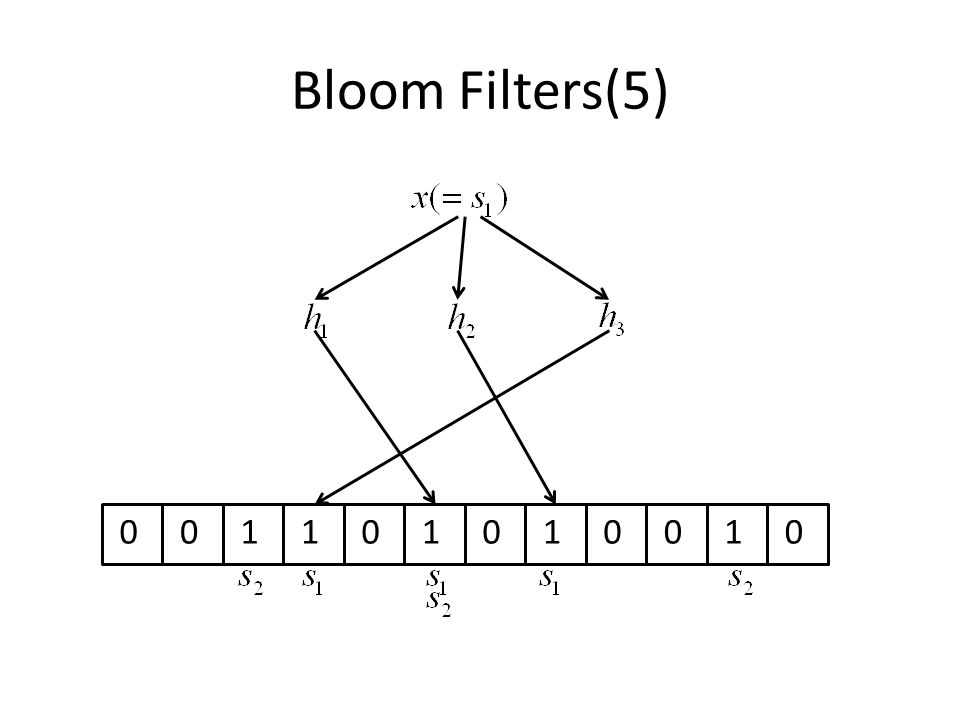
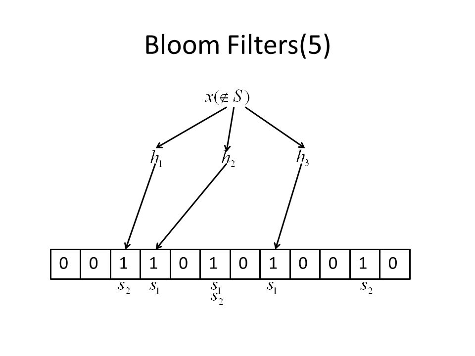
16. Bloom Filters(4) To check if an element x is in S, we check whether all array locations are set to 1 If not, clearly x is not in S If all are set to 1, we assume that x is in S. But sometimes it’s wrong ->detail is explained in the next slide There is a probability of false positives

17. Bloom Filters(5) 000000000000 6 11111

18. 00000000000011111

19. 00000000000011111

20. Bloom Filters(6) We can calculate the probability of false positives After all elements of S are hashed into the Bloom filter, the probability that a specific bit is still 0 is, Let. To simplify the analysis, let fraction of p of the entries are still 0 after all of the elements S are hashed

21. Bloom Filters(7) The probability of false positives is then Now we use p and to represent the probability that a bit in the Bloom filter is 0 and the probability of false positives Suppose that we are given m and n and wish to optimize the number of hash functions k in order to minimize the false positive probability

22. Bloom Filters(8) Using more hash functions -> more chances to find 0-bit for Using fewer hash functions -> increase the fraction of 0-bits in the array The optimal number of k is easily found by taking derivative

23. Bloom Filters(9) Let, so that and minimizing f is as same as minimizing g Then, and it becomes zero when and g becomes minimum at this point In this case, f becomes

24. Bloom Filters(10) On the other hand, consider f as a function of p. We find From the symmetry of this expression, it is easy to check that minimizes f When f is minimized, the fraction of 0 entries becomes half

25. Random Graph Models(1) There are many NP-hard computational problems defined on graphs -Hamiltonian cycle, independent set, vertex cover… Whether these problems are hard for most inputs or just small function of all graphs To study such questions, random graph models are used

26. Random Graph Models(2) There are two types of undirected random graph (i) :n is the number of vertex and p is the probability. For all possible edges, independently add the edge with probability p (ii) :N is the number of edges. We consider all graphs on n vertices with exactly N edges. There are possible graphs and each selected with equal probability

27. Hamiltonian Cycles (1) Hamiltonian path: a path that traverses each vertex exactly once Hamiltonian cycle: a cycle that traverses each vertex exactly once

28. Hamiltonian Cycles (2) Hamiltonian path

29. Hamiltonian Cycles (2) Hamiltonian cycle

30. Hamiltonian Cycles in Random Graphs By analyzing a simple and efficient algorithm for finding Hamiltonian cycle in random graphs, connection between random graphs and ball- and-bins problems are shown Hamiltonian cycle problem is NP-hard. However, this analysis shows that finding a Hamiltonian cycle is not hard for random graphs. The algorithm is randomized algorithm

31. Rotation(1) This algorithm will make use of a simple operation called a rotation G:undirected graph : a simple path in G : an edge of G Then is also a simple path and the operation from P to P’ is called rotation

32. Rotation(2) rotation of P with the rotation edge P P’

33. Hamiltonian Cycle Algorithm(1) Hamiltonian Cycle Algorithm Input: A graph with n vertices Output: A Hamiltonian cycle or failure 1.Start with a random vertex as the head of path 2.Repeat the following steps until the rotation edge closes a Hamiltonian cycle or the unused-edges list of the head of the path is empty: (a) Let the current path be, where is the head, and be the first edge in the head’s list (b) Remove from the head’s list and u’s list (c) If, for, add to the end of path and make it the head

34. Hamiltonian Cycle Algorithm(2) Hamiltonian Cycle Algorithm (d) Otherwise, if, rotate the current path with and set to be the head. (This step closes the Hamiltonian path if k=n and the chosen edge is ) 3.Return a Hamiltonian cycle if one was found or failure if no cycle was found

35. Hamiltonian Cycle Algorithm(3) head

36. Hamiltonian Cycle Algorithm(3) head

37. Hamiltonian Cycle Algorithm(4) Analyze this algorithm is difficult -once the algorithm views some edges in the edge lists, the distribution of the remaining edges is conditioned Consider the modified algorithm

38. Modified Hamiltonian Cycle Algorithm(3) head (i)

39. Modified Hamiltonian Cycle Algorithm(3) head used unused (ii)

40. Modified Hamiltonian Cycle Algorithm(3) used unused head (ii)

41. Modified Hamiltonian Cycle Algorithm(3) head used unused (iii)

42. Modified Hamiltonian Cycle Algorithm(3) head used unused used unused (iii)

43. Modified Hamiltonian Cycle Algorithm(3) head used unused (iii)

44. Modified Hamiltonian Cycle Algorithm(3) head used unused (iii)

45. Modified Hamiltonian Cycle Algorithm(1) Modified Hamiltonian Cycle Algorithm Input and associated edge lists Output A Hamiltonian cycle or failure 1.Start with a random vertex as the head of the path 2.Repeat the following steps until the rotation edge chose (a)Let the current path be with being the head (b) Excuse i, ii, or iii with probabilities,, and respectively i. Reverse the path, and make being the head

46. Modified Hamiltonian Cycle Algorithm(2) Modified Hamiltonian Cycle Algorithm ii. Choose uniformly at random an edge from used- edges( ); if the edge is, rotate the current path with,and set to the head iii. Select the first edge from unused-edges( ), call. If, for, add to the end of the path and make it the head. Otherwise, if, rotate the current path with and set to be the head (c) Update the used-edges and unused-edges lists appropriately. 3. Return the Hamiltonian cycle or failure

47. Modified Hamiltonian Cycle Algorithm(4) For analysis, the process of making graph is different from Each of the n-1 possible edges connected to a vertex v is initially on the unused-edges list for vertex v independently with some probability q, and they are in a random order Sometimes is on the unused-list of u but it is not on the unused-list of v

48. Modified Hamiltonian Cycle Algorithm(5) Lemma5.15: Let be the head vertex after the t-th step. Then, for any vertex u, as long as at the t-th step there is at least one unused edge available at the head vertex, That is, the head vertex can be thought of as being chosen uniformly at random from all vertices at each step

49. Proof of lemma 5.15(1) can become head only if the path is reversed, so with probability If lies on the path and is in used- edge( ), the probability that is

50. Proof of lemma 5.15(2) In the other case, when an edge is chosen from unused-edges( ), the adjacent vertex is uniform over all the remaining vertices - Think about initial setup of unused edges list of. (i)The list of is determined independently from the list of other vertices

51. Proof of lemma 5.15(2) (ii)Therefore, algorithm doesn’t know the remaining edges in unused-edges( ) Hence any vertex that the algorithm haven’t seen seem to equally likely to connect to any remaining possible neighbors The probability becomes

52. Proof of lemma 5.15(3) Thus, for all vertices,

53. Relationship to coupon collector’s problem(1) When k vertices is left to be added, the probability of finding a new vertex is ->This is same as coupon collector’s problem This part we can solve in about times and Hamiltonian path is made by this step After this, the probability of making the Hamiltonian cycle is and this is also solved in about times Totally Hamiltonian cycle is made in

54. Relationship to coupon collector’s problem(2) More concretely, we can prove the theorem Theorem:5.16 Let be the probability that edge is included to the initial unused-edge list. Then modified Hamiltonian cycle algorithm successfully finds a Hamiltonian cycle in iteration of the repeat loop (step2) with probability We can also prove that a random graph has a Hamiltonian cycle with high probability

55. Proof of theorem 5.16(1) Consider the following two events :The algorithm ran for steps but it failed to construct a Hamiltonian cycle :At least one unused-edges list became empty during iteration To fail, either or must occur. First think about the probability of

56. Proof of theorem 5.16(2) Consider the following two events :The algorithm cannot find Hamiltonian path in steps :The algorithm cannot close Hamiltonian path in steps When is occur, either or is occur

57. Proof of theorem 5.16(3) is same as coupon collector’s problem The probability that any specific coupon hasn’t been found among random coupon is By the union bound, the probability that any coupon type is not found is at most

58. Proof of theorem 5.16(4) Similarly, the probability of becomes Because,

59. Proof of theorem 5.16(5) Next consider about. Consider following two events :At least edges were removed from unused-edges list of at least one vertex :At least one vertex had fewer than edges initially in its unused-edges list For occur, either or must occur

60. Proof of theorem 5.16(6) The probability that a given vertex v is the head of path is, independently at each step Hence the number of times X that v is the head during the steps is the binomial random variable

61. Proof of theorem 5.16(7) Using the Chernoff bound with and, for, we have By taking the union bound over all vertices, the probability becomes

62. Proof of theorem 5.16(8) Bound The expected number of edges Y initially in a vertex’s unused-edges list is at least and from and Chernoff bound, By taking the union bound over all vertices, the probability becomes

63. Proof of theorem 5.16(9) Because, is bounded as follows Hence the probability that the algorithm fail to find Hamiltonian cycle is Now theorem 5.16 is proven

64. For. Corollary5.17:By proper initializing unused- edges list, the algorithm will find Hamiltonian cycle on a graph chosen randomly from with probability wherever Partition the edges of input graph as follows. Let be such that. For edge in the input graph, one of the following three possibilities is executed

65. For (2) (i) place the edge on only u’s unused set with probability (ii) place the edge on only v’s unused set with probability (iii) place the edge on both unused set with probability For any,the probability that placed in the v’s unused edge list for is

66. For (3) Moreover, the probability that is placed on both unused-edges list is ->These two placements are like independent events. If, because and this satisfy the condition of theorem 5.16 Hence by this initializing, the algorithm can be applied for