1. Hash Tables CS 310 – Professor Roch Weiss Chapter 20 All figures marked with a chapter and section number are copyrighted © 2006 by Pearson Addison-Wesley unless otherwise indicated. All rights reserved.

2. Hash tables Suppose we decide that the average cost of O(log N) for operations of a binary search tree are too slow. Hash tables provide a way to insert, delete and find in average O(1) time. Why did we even bother with binary search trees?

3. No free lunch The constant time comes with a cost: Hash table elements have no order, so –visiting according to an ordering property –finding the minimum or maximum elements –etc. are all expensive

4. Foundations of hashing Much like binary search trees, we choose some field of a record to serve as a key. A function maps the key to an index. HashFunction(key) index The index is used in an array and the array entries are sometimes referred to as hash buckets.

5. Hash functions A naïve hash function for a string might build a polynomial from the strings encoding: Example:

6. Hash functions We can index an array by hash function index: Cool + any other information

7. Uh-oh For a 4 character string we need over 268,000,000 entries in the array. We can reduce the size to something manageable by using the modulo operator: 142342124 % 10000 = 2124

8. More about the hash function If we consider the hash function to be a polynomial of variable X, e.g. for strings: we can reduce the number of multiplications by incrementally computing the hash function

9. Overflowing the hash function Consider X=128 as in our previous example for hashing strings and assume that we are using 64 bit unsigned integers: so any 10 character string (and most 9 character strings) would overflow a 64 bit unsigned integer.

10. Resolving hash overflow hash_value = 0 for i = 0 to length(A) hash_value = hash_value*X + encoding(A[i]) Avoids computing X i explicitly, but the sum can still overflow…

11. Resolving hash overflow 1.Apply modulo after each operation hash_value = 0 for i = 0 to length(A) hash_value = /* modulo is expensive */ (hash_value*X + encoding(A[i])) % TableSize 2.Allow overflow. We need to be careful though as long polynomials will shift the first elements of the key out of range.

12. Avoiding overflow

13. Allowing overflow

14. Going to extremes… Here, we have effectively set X in our polynomial to the value 1. What are the implications of this?

15. Collisions Our hash function is no longer unique. If we choose our hash function carefully, this will not happen too often. Nonetheless, we still need to handle it and we will investigate different ways to do so.

16. Linear probing Simple idea: When a collison occurs, look for the next empty hash bucket. use this one hashes to used

17. Linear probing analysis The load factor is defined as Let us assume that 1.Each insertion/access of the hash table is independent of other ones (very naïve assumption) 2.The hash table is large (reasonable assumption)

18. Naïve analysis Assuming independence of probes, the average number of buckets examined in a linear probing insertion is 1/(1-λ) Proof: Pr(empty bucket)=(1- λ). On average, if an event occurs with Pr(event)=p, we need to try 1/p times before we expect to have seen the event with probability 1. So, we should have to try 1/(1- λ) times before we see an empty bucket.

19. Primary clustering Hash insertions and finds are not independent. Results in primary clustering

20. Linear probing complexity Given a loading factor of λ, the number of cells examined in a linear probing insertion is approximately: We will accept this without proof.

21. Analysis of find Unsuccessful find –Same as cost of insertion. Successful find –Same as finding item at time when inserted. –If the bin was unused, only 1 probe is needed. –As more collisions occur, the number of probes increase.

22. Analysis of successful find when primary clustering is present Need to average over all load factors up to the current one:

23. Deletion Cost similar to that of find. We cannot simply delete a node. –Why not?

24. Lazy deletion Instead of clearing an entry, we mark it as deleted. A new insertion may place a new value there and mark it active. Hash bins are either: unused, active, or deleted.

25. Perhaps we can do better… Linear probing is not bad: –Average number of probes for a successful search with a hash table 50% loaded is 2.5. –Begins to be problematic as λ approaches 1 (λ=.90 50.5). –Note that this is independent of the table size. Any algorithm that wishes to reduce this needs must be inexpensive enough that it is cheaper than the small number of probes typically needed.

26. Quadratic probing Basic idea: Scatter the collisions so they do not group near one another Suppose hash(n) = H and bin H is used. –Try (H + i 2 )%TableSize for i = 1, 2, 3, … –Note that linear probing used (H+i)%TableSize for i = 1, 2, 3, … Works best when the table size is a prime number.

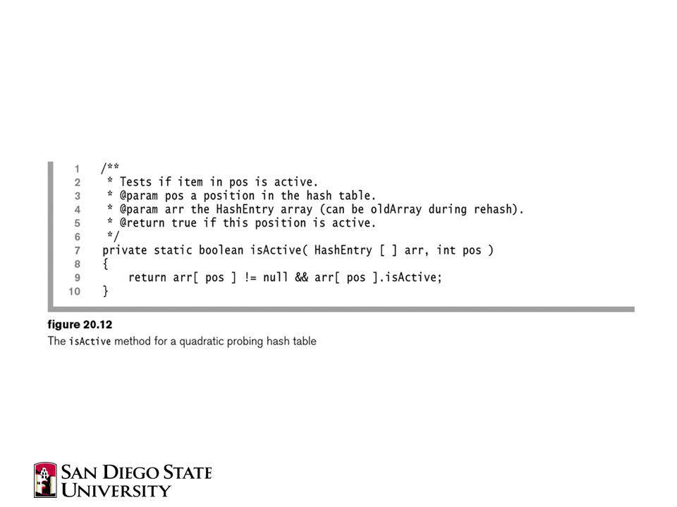
28. Quadratic probing Thm 20.4 – When inserting into a hash table that is at least half empty using quadratic probing, a new element can always be inserted, and no hash bucket is probed more than one time.

29. Insertion with quadratic probing

33. What does this buy us? For a hash table which is less than half full, we have removed the primary clustering. Consequently, we are closer our naïve analysis. On average, when the table is half full, this saves us: –.5 for each insertion –.1 for each successful search In addition, long chains are avoided.

34. What does this cost us? The squared operation and the modulo are relatively expensive given that on average we do not save much. Fortunately, we can improve this...

35. Efficient quadratic probing

36. Effective quadratic probing Multiplication by can be implemented trivially by shift. 2i-1 < M as we never insert into a table that is more than half full. So, H i-1 +2i-1 is either less than H i or is <2M and can be adjusted by subtracting M.

37. More than M/2 entries? Increase the size of the table to the next prime number. Figure 20.7 (read) shows a prime number generation subroutine that is at most O(N.5 logN). This is less than O(N). Copying the table take O(N) time, and has an amortized cost of O(1).

38. Copying the hash bins We do not use the same entries. –Why not? Instead we rehash each item to a new position.

48. Read Read the remainder of the code online and make sure that you understand it. In addition, read the iterator class code.

49. Complexity of quadratic probing No known analysis Eliminates primary clustering Introduces secondary clustering

50. Alternatives Double hashing – Resolve collisions with a second hash function Separate chain hashing – Place collisions on a linked list.

51. Applications Content addressable tables Symbol tables Game playing – Caching state Song recognition