1. Jian Li Institute of Interdisciplinary Information Sciences Tsinghua University Algorithms for Stochastic Geometric and Combinatorial Optimization Problems TexPoint fonts used in EMF. Read the TexPoint manual before you delete this box.: AAA A AA A AAAAAAA lijian83@mail.tsinghua.edu.cn CAS 2015

2. Uncertain Data and Stochastic Model Data Integration and Information Extraction Sensor Networks; Information Networks Probabilistic models in machine learning Sensor IDTemp. 1Gauss(40,4) 2Gauss(50,2) 3Gauss(20,9) …… Probabilistic databases Probabilistic Models in machine learning Stochastic models in operation research

3. Outline Stochastic Models Classical Examples: E[MST] Estimating E[MST] and other statistics Stochastic Combinatorial Optimization: The Poisson Approximation Technique Expected Utility Maximization: The Fourier Decomposition Technique Stochastic Matching: The Linear Programming Technique Conclusion

4. The position of each point is random (non-i.i.d) All pts are independent from each other A popular model in wireless networks/spatial prob databases 0.1 0.5 0.4 Stochastic Geometry Models 0.5 0.3 0.7 0.2 1 0.3 0.2 0.3 Locational uncertainty model

5. The position of each point is random (non-i.i.d) All pts are independent from each other A popular model in wireless networks/spatial prob databases 0.1 0.5 0.4 Stochastic Geometry Models 0.5 0.3 0.7 0.2 1 0.3 0.2 0.3 0.5 0.7 1 0.3 0.5 A realization (aka a possible world) Prob=0.7*1*0.5*0.5*0.3 Locational uncertainty model

6. The position of each point is random (non-i.i.d) All pts are independent from each other A popular model in wireless networks/spatial prob databases 0.1 0.5 0.4 Stochastic Geometry Models 0.5 0.3 0.7 0.2 1 0.3 0.2 0.3 Another realization Prob=0.3*1*0.4*0.5*0.3 Locational uncertainty model 0.4 0.5 0.3 1

7. Stochastic Geometry Models 0.5 0.7 1 0.3 0.5 *(0.7*1*0.5*0.5*0.3) 0.4 0.5 0.3 1 *(0.3*1*0.4*0.5*0.3) + + …… However, this does not give a polynomial time algorithm The stochastic geometry model has been studied in several recent papers for many different problems. [Kamousi, Chan, Suri ‘11] [Afshani, Agarwal, Arge, Larsen, Phillips. ‘11][Agarwal, Cheng, Yi. ‘12] [Abdullah, Daruki, Phillips ‘13] [Suri, Verbeek, Yıldız ‘13] [Li, Wang ‘14] [Agarwal, Har-Peled, Suri, Yıldız, Zhang 14] [Huang, Li ‘15] [Huang, Li, Phillips, Wang ‘15]

8. Stochastic Graph Models The length of each edge is a random variable st

9. Outline Stochastic Models Classical Examples: E[MST] Estimating E[MST] and other statistics Stochastic Combinatorial Optimization: The Poisson Approximation Technique Expected Utility Maximization: The Fourier Decomposition Technique Stochastic Matching: The Linear Programming Technique Conclusion

10. A classic problem in the stochastic graph model A undirected graph with n nodes The length of each edge: i.i.d. Uniform[0,1] Question: What is E[MST]? Ignoring uncertainty (“replace by the expected values” heuristic) each edge has a fixed length 0.5 This gives the WRONG answer 0.5(n-1)

11. A classic problem in the stochastic graph model

12. N points: i.i.d. uniform[0,1]×[0,1] Question: What is E[MST] ? Answer: A classic problem in the stochastic geometry model

13. The problem is similar, but the answer is not similar………… A classic problem in the stochastic geometry model

14. Outline Stochastic Models Classical Examples: E[MST] Estimating E[MST] and other statistics Stochastic Combinatorial Optimization: The Poisson Approximation Technique Expected Utility Maximization: The Fourier Decomposition Technique Stochastic Matching: The Linear Programming Technique Conclusion

15. A Computational Problem The position of each point is random (non-i.i.d) Question: What is E[Closest pair] ? Of Course, there is no close-form formula We need efficient algorithms to compute E[Closest pair] 0.1 0.5 0.4 [Huang, L. ICALP15]

16. Our Results

17. MST over Stochastic Points

18. Monte Carlo Consider the random var: X=0, w.p. 0.999999999999999 X=1, w.p. 0.000000000000001 We need 1000000000000000 in expectation to get a sample of value “1” (just Chernoff Bound) We call X is a nice r.v.

19. Decompose the prob space A carefully chosen random event Y Easy to compute Hopefully, we have

20. #P-hardness Len=1 Len=2 An independent set Cp=2

21. Hierarchical Partition Family (HPF) A minimum spanning tree Edges sorted by their lengths 1 2 3 4 5 6 Level 0 Level 1 Level 2... Level 7

22. Use HPF to decompose the space Events to condition on: Y: the smallest i such that each group in level i contains at most one realized point Level 0 Level 1 Level 2 A realization Y=2 for this realization

23. Use HPF to decompose the space

24. Niceness Only realized points are shown Level i-1 Level i

25. Computing Pr[Y=i]

26. Can be reduced to the permanent approximation problem Consider a slightly simpler problem: Compute Pr[each group gets at most 1 pt]=Per(M) A matching: each group gets at most 1 realized pt M= 111 0.70.20.1 0.40.61 1 0.7 0.2 0.4 0.1 0.6

27. Outline Stochastic Models Classical Examples: E[MST] Estimating E[MST] and other statistics Stochastic Combinatorial Optimization: The Poisson Approximation Technique Expected Utility Maximization: The Fourier Decomposition Technique Stochastic Matching: The Linear Programming Technique Conclusion

28. Existing Techniques A common challenge: How to deal with/ optimize on the distribution of the sum of several random variables. More often seen in the risk-aware setting (linearity of expectation does not help) Previous techniques: Special distributions [Nikolova, Kelner, Brand, Mitzenmacher. ESA’06] [Goel, Indyk. FOCS’99] [Goyal, Ravi. ORL09] ….. Effective bandwidth [Kleinberg, Rabani, Tardos STOC’97] LP [Dean, Goemans, Vondrak. FOCS’04] ….. Discretization [Bhalgat, Goel, Khanna. SODA’11] Characteristic Function + Fourier Series Decomposition [L, Deshpande. FOCS’11] Today: Poisson Approximation [L, Yuan STOC’13]

29. Threshold Probability Maximization Deterministic version: A set of element {e i }, each associated with a weight w i A solution S is a subset of elements (that satisfies some property) Goal: Find a solution S such that the total weight of the solution w(S)= Σ i є S w i is minimized E.g. shortest path, minimal spanning tree, top-k query, matroid base

30. Threshold Probability Maximization Even computing the threshold prob is #P- hard in general! FPTAS exists [Li, Shi, ORL’14]

31. Threshold Probability Maximization Stochastic shortest path : find an s-t path P such that Pr[w(P)<1] is maximized st

32. Our Result

33. Our Results Stochastic shortest path : find an s-t path P such that Pr[w(P)<1] is maximized Previous results Many heuristics Poly-time approximation scheme (PTAS) if (1) all edge weights are normally distributed r.v.s (2) OPT>0.5 [Nikolova, Kelner, Brand, Mitzenmacher. ESA’06] [Nikolova. APPROX’10] Bicriterion PTAS (Pr[w(P) (1-eps)OPT) for exponential distributions [Nikolova, Kelner, Brand, Mitzenmacher. ESA’06] Our result Bicriterion PTAS if OPT= Const st Uncertain length

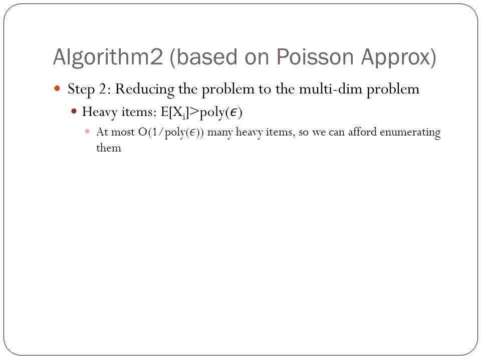
34. Our Results Stochastic knapsack (fixed set version): find a collection S of items such that Pr[w(S) γ and the total profit is maximized Previous results log(1/(1- γ ))-approximation [Kleinberg, Rabani, Tardos. STOC’97] Bicriterion PTAS for exponential distributions [Goel, Indyk. FOCS’99] PTAS for Bernouli distributions if γ = Const [Goel, Indyk. FOCS’99] [Chekuri, Khanna. SODA’00] Bicriterion PTAS if γ = Const [Bhalgat, Goel, Khanna. SODA’11] Our result Bicriterion PTAS if γ = Const (with a better running time than Bhalgat et al.) Stochastic partial-ordered knapsack problem with tree constraints Knapsack, capacity=1 Each item has a deterministic profit and a (uncertain) size

35. Algorithm2 (based on Poisson Approx) Step 1: Discretizing the prob distr (Similar to [Bhalgat, Goel, Khanna. SODA’11], but much simpler) Step 2: Reducing the problem to the multi-dim problem

36. Step 1: Discretizing the prob distr (Similar to [Bhalgat, Goel, Khanna. SODA’11], but simpler) 1 pdf of X i 1 0 0 0 0 0 0 Algorithm2 (based on Poisson Approx)

37. Step 1: Discretizing the prob distr (Similar to [Bhalgat, Goel, Khanna. SODA’11], but simpler) 1 pdf of X i 1 0 0 0 0 0 0 Algorithm2 (based on Poisson Approx)

40. Poisson Approximation

43. Summary

44. Outline Stochastic Models Classical Examples: E[MST] Estimating E[MST] and other statistics Stochastic Combinatorial Optimization: The Poisson Approximation Technique (Adaptive) Stochastic Knapsack Expected Utility Maximization: The Fourier Decomposition Technique Stochastic Matching: The Linear Programming Technique Conclusion

45. Stochastic Knapsack A knapsack of capacity C A set of items, each having a fixed profit Known: Prior distr of size of each item. Each time we choose an item and place it in the knapsack irrevocably The actual size of the item becomes known after the decision Knapsack constraint: The total size of accepted items <= C Goal: maximize E[Profit] [L, Yuan STOC13]

46. Stochastic Knapsack

47. Decision Tree Item 1 Exponential size!!!! (depth=n) How to represent such a tree? Compact solution? Item 2 Item 3Item 7 …..

48. Stochastic Knapsack Still way too many possibilities, how to narrow the search space?

49. Block Adaptive Policies: Process items block by block Items 1,5,7 Items 2,3 Items 3,6 Items 6,8,9 Item 2Item 3 Block Adaptive Policies

50. Items 1,5,7 Items 2,3 Items 3,6 Items 6,8,9 Item 2Item 3 Still exponential many possibilities, even in a single block Block Adaptive Policies Block Adaptive Policies: Process items block by block

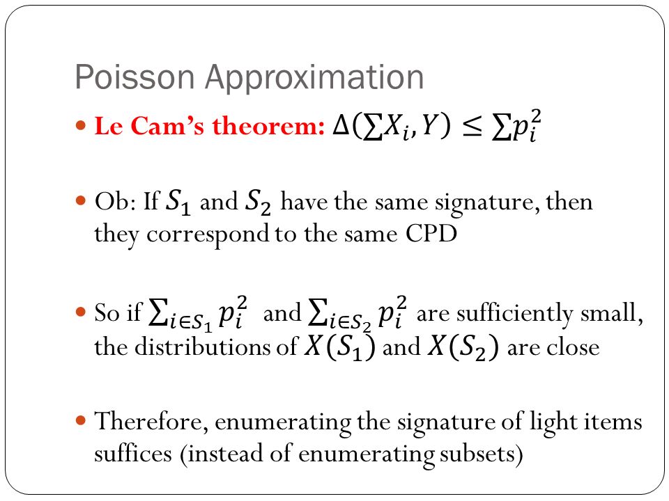
51. Poisson Approximation Each heavy item consists of a singleton block Light items: Recall if two blocks have the same signature, their size distributions are similar So, enumerate Signatures! (instead of enumerating subsets)

52. Outline: Enumerate all block structures with a signature associated with each node (0.4,1.1,0,…) (0,1,1,2.2,…) (5,1,1.7,2,…) (1.1,1,1,1.5,…) (1,1,2,…) (0,1.4,1.2,2.1,…) (0,0,1.5,2,…) -O(1) nodes -Poly(n) possible signatures for each node -So total #configuration =poly(n) Algorithm

53. 2. Find an assignment of items to blocks that matches all signatures – (this can be done by standard dynamic program) Algorithm

54. 2. Find an assignment of items to blocks that matches all signatures – (this can be done by standard dynamic programming) Item 1 (0.2,0.04,0…..) (0.2,0.04,0.1…..) (0.1,0,0…..) (0.1,0.2,0.1…..) (0.15,0,0…..) (0.15,0.2,0.22…..) Item 2Item 3 (0.4,1.1,0,…) (0,1,1,2.2,…) (5,1,1.7,2,…) (1.1,1,1,1.5, …) (1,1,2, …) (0,1.4,1.2,2.1,…) (0,0,1.5,2,…) On any root-leaf path, each item appears at most once Algorithm Item 4 Item 5Item 6

55. Poisson Approximation-Other Applications Prophet inequalities [Chawla, Hartline, Malec, Sivan. STOC10] [Kleinberg, Weinberg. STOC12] Close relations with Secretary problems Applications in multi-parameter mechanism design [L, Yuan STOC13]

56. Outline Stochastic Models Classical Examples: E[MST] Estimating E[MST] and other statistics Stochastic Combinatorial Optimization: The Poisson Approximation Technique Expected Utility Maximization: The Fourier Decomposition Technique Inadequacy of Expected Value Stochastic Matching: The Linear Programming Technique Conclusion

57. Inadequacy of Expected Value Stochastic Optimization Some part of the input are probabilistic Most common objective: Optimizing the expected value Inadequacy of expected value: Unable to capture risk-averse or risk-prone behaviors Action 1: $100 VS Action 2: $200 w.p. 0.5; $0 w.p. 0.5 Risk-averse players prefer Action 1 Risk-prone players prefer Action 2 (e.g., a gambler spends $100 to play Double- or-Nothing)

58. Inadequacy of Expected Value Be aware of risk! St. Petersburg Paradox

59. Outline Stochastic Models Classical Examples: E[MST] Estimating E[MST] and other statistics Stochastic Combinatorial Optimization: The Poisson Approximation Technique Expected Utility Maximization: The Fourier Decomposition Technique Problem definition Stochastic Matching: The Linear Programming Technique Conclusion

60. Expected Utility Maximization Principle Expected Utility Maximization Principle: the decision maker should choose the action that maximizes the expected utility Remedy: Use a utility function Proved quite useful to explain some popular choices that seem to contradict the expected value criterion An axiomatization of the principle (known as von Neumann- Morgenstern expected utility theorem).

61. Problem Definition Deterministic version: A set of element {e i }, each associated with a weight w i A solution S is a subset of elements (that satisfies some property) Goal: Find a solution S such that the total weight of the solution w(S)= Σ i є S w i is minimized E.g. shortest path, minimal spanning tree, top-k query, matroid base

62. Problem Definition Deterministic version: A set of element {e i }, each associated with a weight w i A solution S is a subset of elements (that satisfies some property) Goal: Find a solution S such that the total weight of the solution w(S)= Σ i є S w i is minimized E.g. shortest path, minimal spanning tree, top-k query, matroid base Stochastic version: w i s are independent positive random variable μ (): R + → R + is the utility function (assume lim x → ∞ μ (x)=0) Goal: Find a solution S such that the expected utility E[ μ (w(S))] is maximized

63. Our Results THM: If the following two conditions hold (1) there is a pseudo-polynomial time algorithm for the exact versionof deterministic problem, and (2) μ is bounded by a constant and satisfies Holder condition | μ (x)- μ (y)|≤ C|x-y| α for constant C and α ≥0.5, then we can obtain in polynomial time a solution S such that E[ μ (w(S))]≥OPT- ε, for any fixed ε >0  Exact version: find a solution of weight exactly K  Pseudo-polynomial time: polynomial in K  Problems satisfy condition (1): shortest path, minimum spanning tree, matching, knapsack.

64. Our Results If μ is a threshold function, maximizing E[ μ (w(S))] is equivalent to maximizing Pr[w(S)<1] minimizing overflow prob. [Kleinberg, Rabani, Tardos. STOC’97] [Goel, Indyk. FOCS’99] chance-constrained stochastic optimization problem [Swamy. SODA’11] 1 10 μ (x)

65. Our Results If μ is a threshold function, maximizing E[ μ (w(S))] is equivalent to maximizing Pr[w(S)<1] minimizing overflow prob. [Kleinberg, Rabani, Tardos. STOC’97] [Goel, Indyk. FOCS’99] chance-constrained stochastic optimization problem [Swamy. SODA’11] However, our technique can not handle discontinuous function directly So, we consider a continuous version μ ’ 1 1 1+ δ 0 μ '(x) 1 10 μ (x)

66. Our Results Other Utility Functions Exponential

67. Outline Stochastic Models Classical Examples: E[MST] Estimating E[MST] and other statistics Stochastic Combinatorial Optimization: The Poisson Approximation Technique Expected Utility Maximization: The Fourier Decomposition Technique Algorithm and analysis Stochastic Matching: The Linear Programming Technique Conclusion

68. Our Algorithm Observation: We first note that the exponential utility functions are tractable

69. Our Algorithm Observation: We first note that the exponential utility functions are tractable Approximate the expected utility by a short linear sum of exponential utility Show that the error can be bounded by є

70. Our Algorithm Observation: We first note that the exponential utility functions are tractable Approximate the expected utility by a short linear sum of exponential utility Show that the error can be bounded by є By linearity of expectation

71. Our Algorithm Problem: Find a solution S minimizing

72. Our Algorithm Problem: Find a solution S minimizing Suffices to find a set S such that Opt

73. Our Algorithm Problem: Find a solution S minimizing Suffices to find a set S such that (Approximately) Solve the multi-objective optimization problem with objectives for k=1,…,L Opt

74. Approximating Utility Functions How to approximate μ () by a short sum of exponentials? (with lim μ (x)->0 )

75. Approximating Utility Functions How to approximate μ () by a short sum of exponentials? (with lim μ (x)->0 ) A scheme based on Fourier Series decomposition: For a periodic function f(x) with period 2 ¼ where the Fourier coefficient

76. Approximating Utility Functions How to approximate μ () by a short sum of exponentials? (with lim μ (x)->0 ) A scheme based on Fourier Series decomposition: For a periodic function f(x) with period 2 ¼ where the Fourier coefficient Consider the partial sum (L=2N+1)

77. Approximating The Threshold Function y= ¹ (x) Partial Fourier Series Periodic ! Gibbs Phenomenon Need L=poly(1/ ² ) terms

78. Approximating The Threshold Function y= ¹ (x) Partial Fourier Series Periodic ! Damping Factor : Biased approximation

79. Approximating The Threshold Function y= ¹ (x) Partial Fourier Series Periodic ! Damping Factor : Biased approximation Initial Scaling : Unbiased Apply Fourier series expansion on

80. Approximating The Threshold Function y= ¹ (x) Partial Fourier Series Periodic ! Damping Factor : Biased approximation Initial Scaling : Unbiased Extending the func. Unbiased and better quality around origin

81. The Multi-objective Optimization Want to find a set S such that (Approximately) Solve the multi-objective optimization problem with objectives for i=1,…,L (Similar to [Papadimitriou, Yannakakis FOCS’00]) Each element e has a multi-dimensional weight

82. The Multi-objective Optimization Discretize the vector Enumerate all possible 2L-dimensional vector A (poly many) Think A as the approximate version of Check if there is any feasible solution S such that We use the pseudo-poly algorithm for the exact problem

83. Summary We need L=poly(1/ ² ) terms We solve an O(L) dim optimization problem The overall running time is This improves the running time in [Bhalgat, Goel, Khanna. SODA’11]

84. Extension: Multi-dimensional Weights Stochastic Multidimensional Knapsack: Each element e is associated with a random vector (entries can be correlated) d =O(1) Each element e is associated with a profit p e Objective: Find a set S of items such that and the total profit  is maximized Our result: We can find a set S of items in poly time such that the total profit is at least (1- ² ) of the optimum and

85. Extension: Multi-dimensional Weights Consider the 2-dimensional utility function Consider the rectangular partial sum of the 2d Fourier series expansion A continuous version of the 2d threshold function

86. Discussion Other problems in P? min-cut, matroid base There is no pseudo-poly time algorithm for EXACT-min-cut Why? EXACT-min-cut is strongly NP-hard (harder than MAX-CUT) It is a long standing open problem whether there is a pseudo- poly-time algo for EXACT-matroid base Can we get the same result for these problems? Not for min-cut Consider a deterministic instance where MAX-CUT=1 μ 1 0.878

87. Discussion (1) Monotone and Lipschitz nonincreasing utility function (2) [LY’13] PTAS for the deterministic multi-dimensional version then we can obtain S such that E[ μ (w(S))]≥OPT- ε, for any fixed ε >0. Deterministic multi-dimensional version: Each edge e has a weight (const dim) vector v e. Given a target vector V, find a feasible set S s.t. v(S)<=V A PTAS should either return a feasible set S such that v(S)<=(1+ ε )V or claim that there is no feasible set S such that v(S)<=V

88. Discussion KNOWN: Pseudo-poly for EXACT-A => PTAS for MulDim-A [Papadimitriou, Yannakakis FOCS’00] PTAS for MulDim-MinCut [Armon, Zwick Algorithmica06] PTAS for MulDim-Matroid Base [Ravi, Goemans SWAT96] Pseudo-poly for EXACT PTAS for MulDim Shortest path, Matching, MST, Knapsack Min-cut Matroid base?

89. Open Problems OPEN: Can we extend the technique to the adaptive problem (considered in [Dean,Geomans,Vondrak, FOCS’04 ] [Bhalgat, Goel, Khanna. SODA’11] )? OPEN: Can we get a PTAS? (with a multiplicative error) Even for optimizing the overflow probability Consider maximization problems and increasing utility functions Optimizing or For and, see [Kleinberg, Rabani, Tardos. STOC’97], [Goel, Guha, Munagala PODS’06]

90. Outline Stochastic Models Classical Examples: E[MST] Estimating E[MST] and other statistics Stochastic Combinatorial Optimization: The Poisson Approximation Technique Expected Utility Maximization: The Fourier Decomposition Technique Stochastic Matching: The Linear Programming Technique Conclusion

91. Problem Definition Stochastic Matching [Chen, Immorlica, Karlin, Mahdian, and Rudra. ’09] Given: A probabilistic graph G(V,E). Existential prob. p e for each edge e. Patience level t v for each vertex v. Probing e=(u,v): The only way to know the existence of e. We can probe (u,v) only if t u >0, t v >0. If e indeed exists, we should add it to our matching. If not, t u =t u -1, t v =t v -1.

92. Problem Definition Output: A strategy to probe the edges Edge-probing: an (adaptive or non-adaptive) ordering of edges. Matching-probing: k rounds; In each round, probe a set of disjoint edges Objectives: Unweighted: Max. E[ cardinality of the matching]. Weighted: Max. E[ weight of the matching].

93. Motivations Online dating Existential prob. p e : estimation of the success prob. based on users’ profiles.

94. Motivations Online dating Existential prob. p e : estimation of the success prob. based on users’ profiles. Probing edge e=(u,v) : u and v are sent to a date.

95. Motivations Online dating Existential prob. p e : estimation of the success prob. based on users’ profiles. Probing edge e=(u,v) : u and v are sent to a date. Patience level: obvious.

96. Motivations Kidney exchange Existential prob. p e : estimation of the success prob. based on blood type etc. Probing edge e=(u,v) : the crossmatch test (which is more expensive and time-consuming).

97. Our Results Previous results for unweighted version [Chen et al. ’09]: Edge-probing: Greedy is a 4-approx. Matching-probing: O(log n)-approx. A simple 8-approx. for weighted stochastic matching. For edge-probing model. Can be generalized to set packing. An improved 3-approx. for bipartite graphs and 4-approx. for general graphs based on dependent rounding [Gandhi et al. ’06]. For both edge-probing and matching-probing models. This implies the gap between the best matching-probing strategy and the best edge- probing strategy is a small const.

98. Our Results Previous results for unweighted version [Chen et al. ’09]: Edge-probing: Greedy is a 4-approx. Matching-probing: O(log n)-approx. A simple 8-approx. for weighted stochastic matching. For edge-probing model. Can be generalized to set/hypergraph packing. An improved 3-approx. for bipartite graphs and 4-approx. for general graphs based on dependent rounding [Gandhi et al. ’06]. For both edge-probing and matching-probing models. This implies the gap between the best matching-probing strategy and the best edge- probing strategy is a small const.

99. Our Results Previous results for unweighted version [Chen et al. ’09]: Edge-probing: Greedy is a 4-approx. Matching-probing: O(log n)-approx. A simple 8-approx. for weighted stochastic matching. For edge-probing model. Can be generalized to set/hypergraph packing. An improved 3-approx. for bipartite graphs and 4-approx. for general graphs based on dependent rounding [Gandhi et al. ’06]. For both edge-probing and matching-probing models. This implies the gap between the best matching-probing strategy and the best edge- probing strategy is a small const.

100. Stochastic online matching A set of items and a set of buyer types. A buyer of type b likes item a with probability p ab. G(buyer types, items): Expected graph) The buyers arrive online. Her type is an i.i.d. r.v.. The algorithm shows the buyer (of type b) at most t items one by one. The buyer buys the first item she likes or leaves without buying. Goal: Maximizing the expected number of satisfied users. 1 1 1 1 1 0.9 1 0.5 0.6 0.9 0.2 Expected graph

101. Stochastic online matching This models the online AdWords allocation problem. This generalizes the stochastic online matching problem of [Feldman et al. ’09, Bahmani et al. ’10, Saberi et al ’10] where p e ={0,1}. We have a 4.008-approximation.

102. Approximation Ratio We compare our solution against the optimal (adaptive) strategy (not the offline optimal solution). An example: … t=1 p e= 1/n E[offline optimal] = 1-( 1-1/n) n ≈ 1-1/e E[any algorithm] = 1/n

103. A LP Upper Bound Variable y e : Prob. that any algorithm probes e. At most 1 edge in ∂(v) is matched At most t v edges in ∂(v) are probed x e : Prob. e is matched

104. A Simple 8-Approximation An edge (u,v) is safe if t u >0, t v >0 and neither u nor v is matched Algorithm: Pick a permutation π on edges uniformly at random For each edge e in the ordering π, do: If e is not safe then do not probe it. If e is safe then probe it w.p. y e / α.

105. A Simple 8-Approximation Analysis: Lemma: For any edge (u,v), at the point when (u,v) is considered under π, Pr(u loses its patience) ≤1/2 α. Proof: Let U be #probes incident to u and before e. By the Markov inequality:

106. A Simple 8-Approximation Analysis: Lemma: For any edge e=(u,v), at the point when (u,v) is considered under π, Pr(u is matched) ≤1/2 α. Proof: Let U be #matched edges incident to u and before e. By the Markov inequality:

107. A Simple 8-Approximation Analysis: Theorem: The algorithm is a 8-approximation. Proof: When e is considered, Pr(e is not safe) ≤ Pr(u is matched)+ Pr(u loses its patience)+ Pr(v is matched)+ Pr(v loses its patience) ≤ 2/ α Therefore, Recall Σ e w e y e p e is an upper bound of OPT

108. An Improved Approx. – Bipartite Graphs Algorithm: y ← Optimal solution of the LP. y’ ← Round y to an integral solution using dependent rounding [Gandhi et al. 06] and Let E’= {e | y’ e =1}. (Marginal distribution) Pr(y’ e =1)=y e ; (Degree preservation) Deg E’ (v) ≤ t v ; (Recall Σ e in  v  y e ≤ t v ) (Negative Correlation). Probe the edges in E’ in random order. for any o For matching-probe model: o M 1, …, M h ← Optimal edge coloring of E’. o Probe {M 1, …,M h } in random order.

109. An Improved Approx. – Bipartite Graphs Analysis (sketch): We show Pr[e is probed] >= O(1)y e Assume we have chosen E’. Consider a particular edge e=(u,v). Let B(e, π ) be the set of incident edges that appear before e in the random order π. We claim that

110. An Improved Approx. – Bipartite Graphs Analysis cont: To see Consider this random experiment: For each edge in,,we pick a random real a e in [0,1]. This produces a uniformly random ordering. Let r.v. A f = (1-p f ) if f goes before e, and A f =1 o.w. Then, we consider

111. An Improved Approx. – Bipartite Graphs Analysis cont: Define to be the optimal value of We can show is convex and decreasing on r minimize

112. An Improved Approx. – Bipartite Graphs Analysis cont: Marginal Prob. If p max is 1, =3.

113. An Improved Approx. – Bipartite Graphs Analysis cont: Marginal Prob. Convexity. If p max is 1, =3.

114. An Improved Approx. – Bipartite Graphs Analysis cont: Marginal Prob. Convexity. Negative correlation.

115. An Improved Approx. – General Graphs Algorithm: (x,y) ← Optimal solution of the LP. Randomly partition vertices into A and B. Run the previous algorithm on the bipartite graph G(A,B). Thm: It is a 2/ ρ (1)-approximation. If p max → 1, the ratio tends to 4. If p max → 0, the ratio tends to 2/(1-1/e) ≈3.15

116. Final Remarks and Open Questions Recently, Adamczyk has proved that the greedy algorithm is a 2- approximation for the unweighted version. Better approximations? (Unweighted: 2; Weighted bipartite: 3; Weighted: 4). Can we get anything better than 2 (even without patience parameter)? We recently obtained a PTAS if G is a tree Hardness? Any lower bound?

117. Conclusion Replacing the input random variable with its expectation typically is NOT the right thing to do Carry the randomness along the way and optimize the expectation of the objective We can often reduce the stochastic optimization problem (with independent random variables) to a constant dimensional packing problem Stochastic optimization problems with dependent random variables are typically extremely hard (i.e., inapproximable) Many interesting problems in the stochastic models

118. Many Other Problems Stochastic geometry models Nearest neighbor queries [Afshani, Agarwal, Arge, Larsen, Phillips. ‘11] Range queries [Li, Wang ‘14] [Agarwal, Har-Peled, Suri, Yıldız, Zhang 14] Coresets [Abdullah, Daruki, Phillips ‘13] [Huang, Li, Phillips, Wang ‘15] Shape fitting (minimum enclosing ball, cylinder etc.) [Feldman, Munteanu, Sohler 14] [Huang, Li, Phillips, Wang ‘15]

119. Thanks lijian83@mail.tsinghua.edu.cn