Download presentation
Presentation is loading. Please wait.

1
Describing Relationships

2
Least-Squares Regression A method for finding a line that summarizes the relationship between two variables Only in a specific setting Different people may draw different lines by eye on a scatterplot. This gives us an exact procedure/formula

3
Regression Line A straight line that describes how a response variable y changes as an explanatory variable x changes Unlike correlation, we must have explanatory and response variables Often use regression line to make a prediction No line will pass through all the points We use the line to predict y from x, so we want a line that is as close as possible to the points in the vertical direction Regression line makes the vertical distance of the point in the scatterplot as small as possible

4
Example 3.8 Page 150

5
Least-squares regression line (LSRL) A model used when the data shows a linear trend The line that makes the sum of the squares of the vertical distances of the data point from the line as small as possible Can’t just go with what visually looks like the best fit Picture on page 151 (shown on next 2 slides) Error = observed – predicted
 A model used when the data shows a linear trend The line that makes the sum of the squares of the vertical distances of the data point from the line as small as possible Can’t just go with what visually looks like the best fit Picture on page 151 (shown on next 2 slides) Error = observed – predicted")
8
LSRL Equation: Slope: Intercept: Notice these use and s

9
Why do we use ? y denotes observed value (read “y hat”) denotes predicted value When you are solving regression problems, make sure you are careful to distinguish between y and
 denotes predicted value When you are solving regression problems, make sure you are careful to distinguish between y and.")
10
Two necessary conditions Every least-squares regression line passes through the point the slope of the least-squares line is equal to the product of the correlation and the quotient of the standard deviations: Commit these two facts to memory and you will be able to find equations of least-squares lines

11
Constructing Least-Squares Regression without Data Use the following data to construct the equation for the least-squares line:

12
Constructing LSRL

13
The magic of the calculator The calculator will find the information for you 8:LinReg(a+bx) Make sure that your r and values appear When you write your equation, do not forget to use,this means predicted value To plot the line on the scatterplot by hand, use the equation to find for two values of x, one near each end of the range of x in the data
 Make sure that your r and values appear When you write your equation, do not forget to use,this means predicted value To plot the line on the scatterplot by hand, use the equation to find for two values of x, one near each end of the range of x in the data")
14
Warm up Find the equation of the Least Squares Regression Line (LSRL) that models the relationship between corrosion and strength and the correlation coefficient. Use the prediction model (LSRL) to determine the following: What is the predicted strength of concrete with a corrosion depth of 25mm? What is the predicted strength of concrete with a corrosion depth of 40mm?
 to determine the following: What is the predicted strength of concrete with a corrosion depth of 25mm. What is the predicted strength of concrete with a corrosion depth of 40mm .")
15
r tells us there is a strong, negative, LINEAR relationship between depth of corrosion and strength of concrete. b (the slope) tells us that for every increase of 1 mm in depth of corrosion, we PREDICT a 0.28 decrease in strength of the concrete. a (the y-intercept or constant) tells us the initial PREDICTED strength
 tells us that for every increase of 1 mm in depth of corrosion, we PREDICT a 0.28 decrease in strength of the concrete. a (the y-intercept or constant) tells us the initial PREDICTED strength.")
17
How to add a regression line to your scatterplot on TI-84

18
Explanatory vs. Response The Distinction Between Explanatory and Response variables is essential in regression. Switching the distinction results in a different least-squares regression line. Note: The correlation value, r, does NOT depend on the distinction between Explanatory and Response.

19
Computer output for LSRL

20
Coefficient of Determination The coefficient of determination, r 2, describes the percent of variability in y that is explained by the linear regression on x. 71% of the variability in death rates due to heart disease can be explained by the LSRL on alcohol consumption. That is, alcohol consumption provides us with a fairly good prediction of death rate due to heart disease, but other factors contribute to this rate, so our prediction will be off somewhat.

21
Coefficient of Determination (r 2 ) r vs. r 2 Correlation: strength of association Coefficient of determination: how successful you are Some computer output calls it R-sq

22
Calculating r 2 r 2 = SST: sum of the squares about the mean SSE: sum of the squares for error Interpretation: the proportion of the total sample variability that is explained by the least-square regression of y on x

23
Example 3.13 page 164 r = 0.9953 r 2 = 0.9906 This means over 99% of the variation in gas consumption is accounted for by the linear relationship with degree-days.

24
r = 7842 r 2 = 0.6150 This means that the linear relationship between distance and velocity explains about 61.5% of the variation in either variable.

25
Warmup Sarah’s parents are concerned that she seems short for her age. Their doctor has the following record of Sarah’s height: Age (months):364851545760 Height (cm): 869091939495 a) Make a scatterplot of these data. b) Using your calculator, find the equation of the least- squares regression line of height on age. c) Use your regression line to predict Sarah’s height at age 40 years (480 months). Convert your prediction to inches (2.54 cm = 1 inch). Does this make sense? Explain.
: Height (cm): a) Make a scatterplot of these data. b) Using your calculator, find the equation of the least- squares regression line of height on age. c) Use your regression line to predict Sarah’s height at age 40 years (480 months). Convert your prediction to inches (2.54 cm = 1 inch). Does this make sense. Explain..")
26
Residuals The difference between the observed value of the response variable and the value predicted by the regression line Residual = observed y – predicted y = The mean of the residuals is always 0 Sometimes not exact on calculator due to roundoff error

28
Example 3.14 page 167

30
Predict the Gesell Score for a child who first spoke at 15 months. What is the residual? The residual is positive because it lies above the line

31
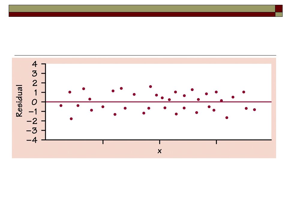
Residual Plot This line corresponds to the regression line from before

32
Residual plots A scatterplot of the regression residuals against the explanatory variables Help us to assess the fit of a regression line

33
Calculator can produce graph of residuals (page 174)
")
34
Some facts: A good residual plot has a uniform scatter of points above and below the line y = 0 There should be no systematic pattern or unusual individual observations A curved pattern shows that the relationship is not linear Increasing or decreasing the spread about the line as x increases indicates that prediction of y will be less accurate for larger x

38
More facts: Individual points with large residuals are outliers in the vertical (y) direction because they lie far from the line that describes the overall pattern Individual points that are extreme in the x direction may not have large residuals, but they can be very important
 direction because they lie far from the line that describes the overall pattern Individual points that are extreme in the x direction may not have large residuals, but they can be very important")
39
Influential Observations Outliers: an observation that lies outside the overall pattern of the other observations Influential point: one that, if removed, would markedly change the result of the calculation outliers in the x direction are often influential for the least-squares regression line Often have small residuals because they pull the regression line towards themselves can see what removal of such a point does to the line on page 172 (next slide) Child 19 has less influence than child 18
 Child 19 has less influence than child 18")
41
Outliers/Influential Points Does the age of a child’s first word predict his/her mental ability? Consider the following data on (age of first word, Gesell Adaptive Score) for 21 children. Does the highlighted point markedly affect the equation of the LSRL? If so, it is “influential”. Test by removing the point and finding the new LSRL. Influential?
 for 21 children. Does the highlighted point markedly affect the equation of the LSRL. If so, it is influential . Test by removing the point and finding the new LSRL. Influential .")
42
Interpolation: predicting a value within the parameter of the data given Extrapolation: predicting a value outside the parameter of the data given Beware of extrapolation!

43
Applets Adding a point to a scatterplot Adding a point to a scatterplot Regression by eye Regression by eye Regression line and residuals Regression line and residuals

Similar presentations


 Weight (lb) 53 80 67.5 344 72 416>")


 of the.>")

>")
