1. Chapter 3 Section 3.1 Examining Relationships

2. Continue to ask the preliminary questions familiar from Chapter 1 and 2 What individuals do the data describe? What are the variables? How are the variables measured? Are all the variables quantitative or is at least one a categorical variable? Do you want to explore the nature of the relationship or do you think some of the variables explain or cause the changes in others?

3. bivariate involving two variables, especially, when attempting to show a correlation between two variables, the analysis is said to be bivariate

4. When working with bivariate data, each variable plays a different role. One variable is the explanatory or predictor variable, while the other is the response variable.

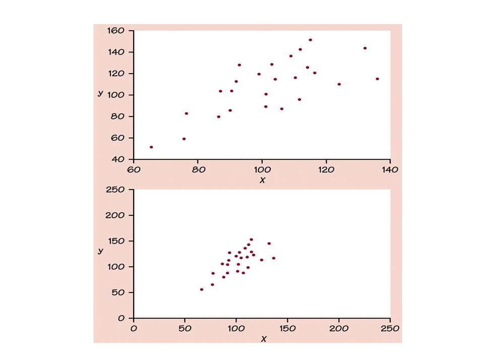
5. Bivariate data is graphed on a scatterplot with an x-axis (horizontal) and y-axis (vertical). The explanatory variable is graphed on the horizontal, and the response variable is graphed on the vertical. A scatterplot is a picture of the association between two variables.

6. Do Problem 3.2 pg 123.

7. Tips for drawing scatterplots Scale the horizontal and vertical axes. The intervals must be uniform. If the scale does not begin at zero use the // symbol to indicate a break Label both axes If given a grid, use a scale so that your plot utilizes the whole grid. Don’t compress the plot into one corner of the grid.

8. To analyze a scatterplot, describe the data in terms of: Direction (positive or negative) Form (linear, clustered, curve) Scatter or strength ( recognize positive or negative association and linear patterns) Outlier (deviation from the overall pattern)

13. Do the following problems as example problems 3.6 pg. 125 3.10 pg 129 3.22 pg 139

14. End of Section 3.1

15. CHAPTER 3 SECTION 3.2

16. Lesson 3.2 Correlation Correlation is given by the following equation: Correlation measures the direction and strength of the linear relationship between two quantitative variables. It is the average of the products of the standardized values.

17. The correlation computed from the sample data measures the direction and strength of the linear relationship between two quantitative variables. The symbol for the sample correlation coefficient is r. The range of the correlation is from -1 to +1. When r is close to +1, there is a strong positive linear relationship between the variables. When r is close to -1, there is a strong negative relationship between the variables. When there is no linear relationship or only a weak relationship, the value of r will be close to 0. The correlation is not resistant. It is strongly affected by outliers.

20. If women always married men who were two years older than themselves, what would be the correlation between the ages of husband and wife?

21. The gas mileage of an automobile first increases and then decreases as the speed increases. This relationship is very regular as shown by the following data on speed (miles per hour) and the mileage (miles per gallon): Speed: 20 30 40 50 60 MPG: 24 28 30 28 24 Make a scatter plot; calculate r.

22. End of Section 3.2

23. Section 3.3 Least Squares Regression

24. LEAST-SQUARES REGRESSION Given a scatter plot, one must be able to draw the line of best fit. Best fit means that the sum of the squares of the vertical distances from each point to the line is minimized.

25. When the scatterplot appears linear, the line of best fit is the Least-Squares Regression Line (LSRL).

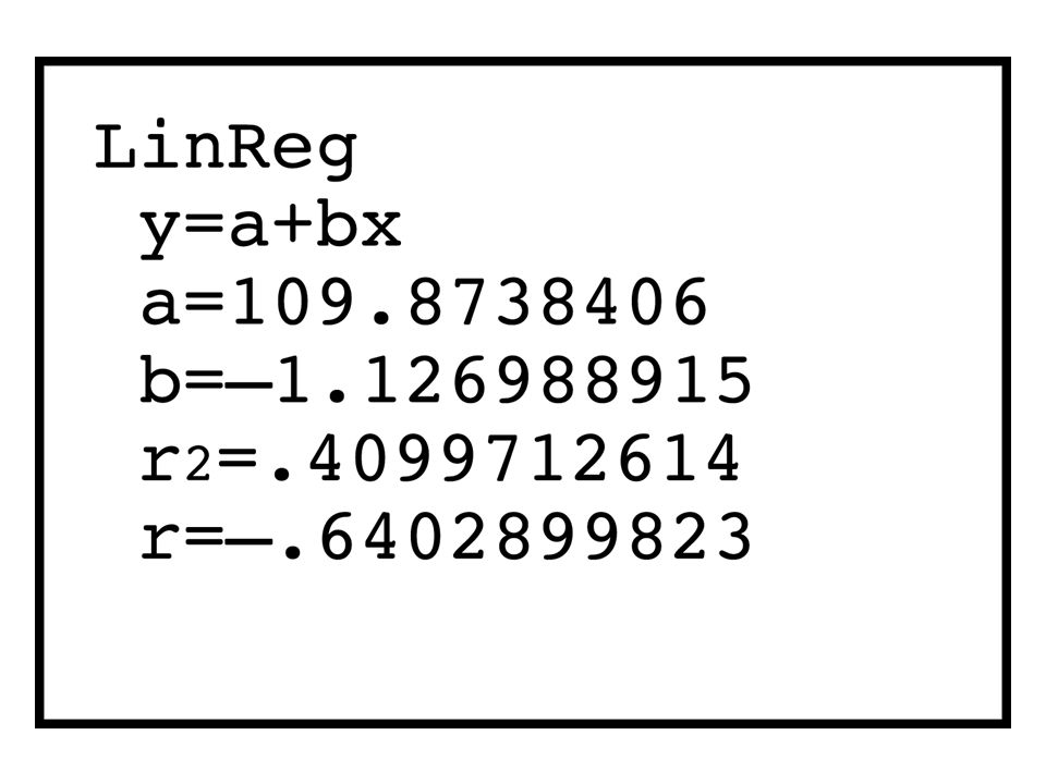
26. Equation of the Least-Squares Regression Line (LSRL) is read “y-hat” and means the predicted value of y. a is the y-intercept. b is the slope. is on the LSRL.

27. Equation for the slope of the LSRL: r is the correlation coefficient. s x if the standard deviation of x. s y is the standard deviation of y.

28. Equation for the y-intercept of the LSRL : a is the y-intercept. is the mean of the y-values. is the mean of the x-values.

31. y: observed value y bar: mean of observed values ŷ: predicted values

32. Do problem 3.38 pg 158 refer back to data in FIG 3.1 pg 127

33. What is ? How do we interpret ? If you know nothing about y’s relationship to x, when you want to predict y, the best you can do is use y-bar. In this case, TOTAL SUM OF SQUARED ERROR :

34. If you know something about the relationship between x and y, then SUM OF SQUARES FOR ERROR:

35. Which is greater, SST or SSE?

36. If x is a poor predictor of y, then the sum of square of deviation about the mean y and the sum of square of deviation about the regression line ŷ would be approximately the same

37. Is the amount of error you eliminated, and is the proportion of error eliminated out of the total error you started with.

39. R 2 The Coefficient of Determination It is, also, known as the coefficient of variation. The coefficient of determination, r 2, is the fraction of the variation in the values of y that is explained by the least-squares regression of y on x.

40. When you report r, give r 2 as a measure of how successful the regression was in explaining the response. When you see r, square it to get a better feel for the strength of the response. Example: r =.7, r 2 =.49. r 2 =.49 means that 49% of the variation in y is explained by the least squares regression of y on x.

41. The correlation between math and verbal SAT scores for this class was.66. What percent of the variation in the verbal scores is explained by the math scores?

42. In a study of the effect of temperature on household heating bills, an investigator said, “Our research shows that about 70% of the variability in the heating units used by a particular house over the years can be explained by outside temperature.” Explain what the investigator meant by this statement. According to this study, what is the correlation between outside temperature and heating bills?

43. RESIDUALS Residual = The mean of the least squares residuals always equals zero. (taking into account round-off error) An effective tool for testing the goodness of fit of a regression line to a bivariate data set is the residual plot.

44. Do problem 3.42 pg 167

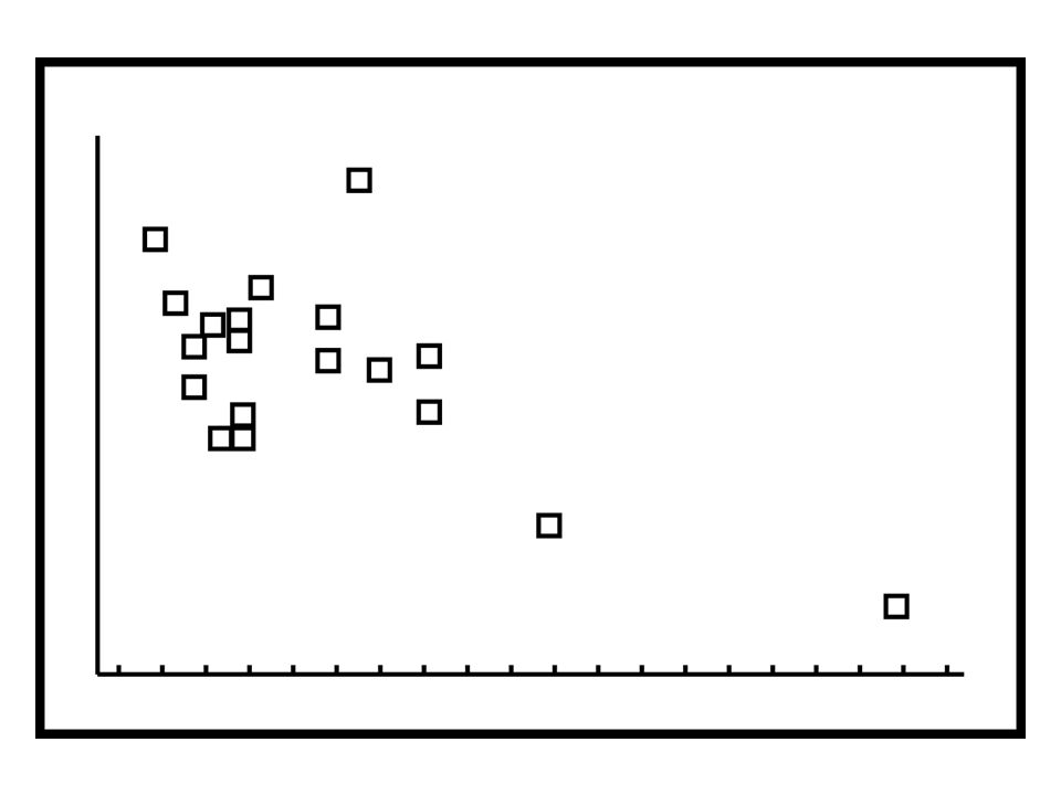
45. RESIDUAL PLOT The residual plot displays the scatterplot of the points If the residual plot shows a random dispersion with no apparent pattern, the LSRL fits the data. If the residual plot shows a curved pattern or fanned pattern, the LSRL is not a good summary for the data

47. When the TI-83 executes a regression model, the residuals are automatically computed and stored in the list RESID. It will be located alphabetically in the NAMES list.

50. Do problem 3.48 which refers back to data in Table 3.4 and the equation in Example 3.14 pg 168.

51. TECHNOLOGY TOOLBOX

56. Analyzing Data for Two Variables

57. End of Chapter 3