Download presentation
Presentation is loading. Please wait.

1
Top-down and bottom-up estimates of North American methane emissions Daniel J. Jacob with Bram Maasakkers, Jianxiong Sheng, Melissa Sulprizio, Alex Turner

2
Ultimate goal of inverse analyses is to improve bottom-up inventories Process-based emission inventory (bottom-up) Atmospheric observations (top-down) prior estimate for inversion correction to bottom-up emissions For this to be successful requires starting from best possible bottom-up inventory including: High-quality representation of processes Detailed documentation on source types, activity rates, emission factors Complete error characterization Spatially and temporally resolved information for testing with atmospheric data
 Atmospheric observations (top-down) prior estimate for inversion correction to bottom-up emissions For this to be successful requires starting from best possible bottom-up inventory including: High-quality representation of processes Detailed documentation on source types, activity rates, emission factors Complete error characterization Spatially and temporally resolved information for testing with atmospheric data")
3
Inverse studies using EDGAR emission inventory as prior find the need for large corrections SCIAMACHY (2004) [Wecht et al., 2014] Correction factors vs. EDGAR NOAA surface/aircraft (2007-2009) [Miller et al., 2013] GOSAT (2009-2011) [Turner et al., 2015] EDGAR has 0.1 o x0.1 o spatial resolution but is based on crude IPCC Tier 1 methods Using a better bottom-up inventory with highly resolved data by source types would -Improve the quality of the inversions -Facilitate interpretation of inversion results -Contribute to improvement of the bottom-up inventory and advance knowledge
![Inverse studies using EDGAR emission inventory as prior find the need for large corrections SCIAMACHY (2004) [Wecht et al., 2014] Correction factors vs.](http://images.slideplayer.com/36/10596122/slides/slide_3.jpg "EDGAR NOAA surface/aircraft ( ) [Miller et al., 2013] GOSAT ( ) [Turner et al., 2015] EDGAR has 0.1 o x0.1 o spatial resolution but is based on crude IPCC Tier 1 methods Using a better bottom-up inventory with highly resolved data by source types would -Improve the quality of the inversions -Facilitate interpretation of inversion results -Contribute to improvement of the bottom-up inventory and advance knowledge.")
4
enteric fermentation (6.7) rice (0.4) onshore (0.9) offshore (0.6) Natural gas 6.2 production (2.0) processing (0.9) transmission (2.1) distribution (1.2) Oil 1.5 Coal mines 3.2 Agriculture 9.6 landfills (4.9) wastewater (0.6) Waste 5.5 Other 1.4 US EPA [2014] US EPA National Greenhouse Gas Inventory for methane (2012)
![enteric fermentation (6.7) rice (0.4) onshore (0.9) offshore (0.6) Natural gas 6.2 production (2.0) processing (0.9) transmission (2.1) distribution (1.2) Oil 1.5 Coal mines 3.2 Agriculture 9.6 landfills (4.9) wastewater (0.6) Waste 5.5 Other 1.4 US EPA [2014] US EPA National Greenhouse Gas Inventory for methane (2012)](http://images.slideplayer.com/36/10596122/slides/slide_4.jpg "enteric fermentation (6.7) rice (0.4) onshore (0.9) offshore (0.6) Natural gas 6.2 production (2.0) processing (0.9) transmission (2.1) distribution (1.2) Oil 1.5 Coal mines 3.2 Agriculture 9.6 landfills (4.9) wastewater (0.6) Waste 5.5 Other 1.4 US EPA [2014] US EPA National Greenhouse Gas Inventory for methane (2012)")
5
enteric fermentation (6.7) rice (0.5) onshore (2.1) offshore (0.2) Natural gas 6.9 production (4.4) processing (0.9) transmission (1.1) distribution (0.5) Oil 2.3 Coal mines 2.9 Agriculture 9.7 landfills (6.9) wastewater (0.6) Waste 7.6 Other 0.8 US EPA [2016] US EPA National Greenhouse Gas Inventory for methane (2012)
![enteric fermentation (6.7) rice (0.5) onshore (2.1) offshore (0.2) Natural gas 6.9 production (4.4) processing (0.9) transmission (1.1) distribution (0.5) Oil 2.3 Coal mines 2.9 Agriculture 9.7 landfills (6.9) wastewater (0.6) Waste 7.6 Other 0.8 US EPA [2016] US EPA National Greenhouse Gas Inventory for methane (2012)](http://images.slideplayer.com/36/10596122/slides/slide_5.jpg "enteric fermentation (6.7) rice (0.5) onshore (2.1) offshore (0.2) Natural gas 6.9 production (4.4) processing (0.9) transmission (1.1) distribution (0.5) Oil 2.3 Coal mines 2.9 Agriculture 9.7 landfills (6.9) wastewater (0.6) Waste 7.6 Other 0.8 US EPA [2016] US EPA National Greenhouse Gas Inventory for methane (2012)")
6
Constructing a gridded version of the EPA national inventory Greenhouse Gas Reporting Program: large point sources (coal, waste, oil/gas) report emissions to EPA Additional data for locations of oil/gas wells, stations, pipelines, coal mines, landfills, wastewater plants… Data for livestock, manure management, rice at sub-county level (USDA + EPA) Maasakkers et al., in prep. Reconciliation to EPA state/national totals for each source subcategory 0.1 o x0.1 o gridded information Gridded version of EPA inventory 0.1 o x0.1 o monthly resolution detailed breakdown by source types scale-dependent error characterization matches state/national totals from EPA Process-level emission factors including monthly variation A joint Harvard-EPA project 22 layers of data with M. Weitz, T. Wirth, C Hight, L Hockstadt (EPA)
.")
7
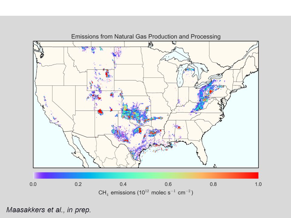
Maasakkers et al., in prep.

11
Gridded EPA anthropogenic methane emissions for 2012 Maasakkers et al., in prep.

12
EDGAR v4.2 anthropogenic methane emissions for 2008

13
Difference between gridded EPA and EDGAR v4.2 Maasakkers et al., in prep.

14
Differences in spatial allocation between EPA and EDGAR impact inversion results and source attribution

15
Using EDF Barnett Shale inventory as “truth” to characterize scale-dependent EPA inventory errors For each source type, least-squares fit to error model over grid squares x: relative error EPA error std dev. at location x displacement error Maasakkers et al., in prep. Lyon et al. [2015] EPA

16
Error standard deviation for 0.1 o ×0.1 o and coarser grids Livestock Landfills Wastewater Natural gas Petroleum Maasakkers et al., in prep. National Grid resolution

17
Error evaluation by comparison to CALGEM inventory for California Maasakkers et al., in prep. Most errors are within one standard deviation CALGEM has more precise locations for livestock

18
2.32 Tg CH 4 a -1 Gridded version of ICF national inventory for Canadian oil and gas emissions (2013) Oil production 0.52 Gas production & processing 1.46 Gas transmission 0.29 Gas distribution 0.05 Sheng et al., in prep.
 Oil production 0.52 Gas production & processing 1.46 Gas transmission 0.29 Gas distribution 0.05 Sheng et al., in prep.")
19
Gridded version of IMF national Inventory for Mexican oil and gas emissions (2010) 1.17 Tg CH 4 a -1 Oil production 0.87 Gas production 0.21 Gas transmission 0.05 Gas distribution 0.04 Sheng et al., in prep.
 1.17 Tg CH 4 a -1 Oil production 0.87 Gas production 0.21 Gas transmission 0.05 Gas distribution 0.04 Sheng et al., in prep.")
20
InstrumentAgencyData period Pixel size [km 2 ] CoveragePrecision Low Earth Orbit Solar backscatter SCIAMACHYESA2003-2012 30 60 6 days1.5 % GOSATJAXA2009- 10 10 3 days (sparse)0.7 % TROPOMIESA2016- 7777 1 day0.6% GHGSatGHGSat, Inc.2016-0.05x0.05targets (12x12 km 2 )1-5% GOSAT-2JAXA2018-10x103 days (sparse)0.4% CarbonSatESAproposed 2222 5-10 days0.4% Active (lidar) MERLINDLR/CNES2020- 50 50 monthly1.0% Geostationary GEO-CAPENASAproposed 4444 continental hourly1.0% geoCARBNASAproposed 4545 2-8 hours1.0% SWIR satellite instruments for observing methane
![InstrumentAgencyData period Pixel size [km 2 ] CoveragePrecision Low Earth Orbit Solar backscatter SCIAMACHYESA 60 6 days1.5 % GOSATJAXA 10 3 days (sparse)0.7 % TROPOMIESA 777 1 day0.6% GHGSatGHGSat, Inc x0.05targets (12x12 km 2 )1-5% GOSAT-2JAXA x103 days (sparse)0.4% CarbonSatESAproposed 222 days0.4% Active (lidar) MERLINDLR/CNES 50 monthly1.0% Geostationary GEO-CAPENASAproposed 4444 continental hourly1.0% geoCARBNASAproposed 4545 2-8 hours1.0% SWIR satellite instruments for observing methane](http://images.slideplayer.com/36/10596122/slides/slide_20.jpg "InstrumentAgencyData period Pixel size [km 2 ] CoveragePrecision Low Earth Orbit Solar backscatter SCIAMACHYESA 60 6 days1.5 % GOSATJAXA 10 3 days (sparse)0.7 % TROPOMIESA 777 1 day0.6% GHGSatGHGSat, Inc x0.05targets (12x12 km 2 )1-5% GOSAT-2JAXA x103 days (sparse)0.4% CarbonSatESAproposed 222 days0.4% Active (lidar) MERLINDLR/CNES 50 monthly1.0% Geostationary GEO-CAPENASAproposed 4444 continental hourly1.0% geoCARBNASAproposed 4545 2-8 hours1.0% SWIR satellite instruments for observing methane")
21
InstrumentAgencyData period Pixel size [km 2 ] CoveragePrecision Low Earth Orbit Solar backscatter SCIAMACHYESA2003-2012 30 60 6 days1.5 % GOSATJAXA2009- 10 10 3 days (sparse)0.7 % TROPOMIESA2016- 7777 1 day0.6% GHGSatGHGSat, Inc.2016-0.05x0.05targets (12x12 km 2 )1-5% GOSAT-2JAXA2018-10x103 days (sparse)0.4% CarbonSatESAproposed 2222 5-10 days0.4% Active (lidar) MERLINDLR/CNES2020- 50 50 monthly1.0% Geostationary GEO-CAPENASAproposed 4444 continental hourly1.0% geoCARBNASAproposed 4545 2-8 hours1.0% SWIR satellite instruments for observing methane
![InstrumentAgencyData period Pixel size [km 2 ] CoveragePrecision Low Earth Orbit Solar backscatter SCIAMACHYESA 60 6 days1.5 % GOSATJAXA 10 3 days (sparse)0.7 % TROPOMIESA 777 1 day0.6% GHGSatGHGSat, Inc x0.05targets (12x12 km 2 )1-5% GOSAT-2JAXA x103 days (sparse)0.4% CarbonSatESAproposed 222 days0.4% Active (lidar) MERLINDLR/CNES 50 monthly1.0% Geostationary GEO-CAPENASAproposed 4444 continental hourly1.0% geoCARBNASAproposed 4545 2-8 hours1.0% SWIR satellite instruments for observing methane](http://images.slideplayer.com/36/10596122/slides/slide_21.jpg "InstrumentAgencyData period Pixel size [km 2 ] CoveragePrecision Low Earth Orbit Solar backscatter SCIAMACHYESA 60 6 days1.5 % GOSATJAXA 10 3 days (sparse)0.7 % TROPOMIESA 777 1 day0.6% GHGSatGHGSat, Inc x0.05targets (12x12 km 2 )1-5% GOSAT-2JAXA x103 days (sparse)0.4% CarbonSatESAproposed 222 days0.4% Active (lidar) MERLINDLR/CNES 50 monthly1.0% Geostationary GEO-CAPENASAproposed 4444 continental hourly1.0% geoCARBNASAproposed 4545 2-8 hours1.0% SWIR satellite instruments for observing methane")
22
Observability of regional/point sources from space InstrumentRegional source quantification (Q =72 tons h -1 over 300 300 km 2 ) Barnett Shale Single-pass point source detection threshold (Q min, tons h -1 ) SCIAMACHY1 year averaging time7 GOSAT1 year averaging time7 TROPOMIsingle pass4 GHGSatNA0.2 GOSAT-24 months averaging time4 CarbonSatsingle pass0.8 GEO-CAPE/geoCARB1 hour4 “Super-emitter” point sources observed in Barnett Shale are ~ 1.0 tons h -1 Simple mass balance analysis for source pixels
 Barnett Shale Single-pass point source detection threshold (Q min, tons h -1 ) SCIAMACHY1 year averaging time7 GOSAT1 year averaging time7 TROPOMIsingle pass4 GHGSatNA0.2 GOSAT-24 months averaging time4 CarbonSatsingle pass0.8 GEO-CAPE/geoCARB1 hour4 Super-emitter point sources observed in Barnett Shale are ~ 1.0 tons h -1 Simple mass balance analysis for source pixels")
23
PDFs of 0.1 o x0.1 o and point sources of methane in the US Emission [tons h -1 ] 0.01 1 10 100 0.1 1 10 100 0.1 TROPOMI (single pass) TROPOMI (year) GHGSat (single pass) Cumulative probability distribution function
![PDFs of 0.1 o x0.1 o and point sources of methane in the US Emission [tons h -1 ] TROPOMI (single pass) TROPOMI (year) GHGSat (single pass) Cumulative probability distribution function](http://images.slideplayer.com/36/10596122/slides/slide_23.jpg "PDFs of 0.1 o x0.1 o and point sources of methane in the US Emission [tons h -1 ] TROPOMI (single pass) TROPOMI (year) GHGSat (single pass) Cumulative probability distribution function")
24
Using plume data to better quantify point sources Meandering Gaussian plume (top view) pixels Increase # of pixels but weaker signal Need to invert plume dispersion model What about overlapping plumes? More work is needed! For pixel sizes < 1km, plume structure affects the retrieval (“plume shadow”): plume (front view) Air mass factor depends on plume structure Need 3-D representation of plume
: plume (front view) Air mass factor depends on plume structure Need 3-D representation of plume.")
25
Geostationary satellites in future methane observing system Geostationary orbit allows unique combination of continental-scale mapping high spatial resolution over source regions high temporal frequency for detecting transient sources (super-emitters) Current proposals emphasize continental-scale mapping on hourly time scales… …but this sacrifices precision and compromises detection of transient sources Longer-term staring over selected source regions should be an important component Alternating continental-scale mapping and “special observations” over source regions may be the best strategy
 Current proposals emphasize continental-scale mapping on hourly time scales… …but this sacrifices precision and compromises detection of transient sources Longer-term staring over selected source regions should be an important component Alternating continental-scale mapping and special observations over source regions may be the best strategy")
Similar presentations


, Steven.>")


 Wong.>")


 in-situ network: quantification of urban atmospheric boundary layer greenhouse gas dry mole fraction enhancements 18 th WMO/IAEA.>")

