1. Instructor: Eyal Amir Grad TAs: Wen Pu, Yonatan Bisk Undergrad TAs: Sam Johnson, Nikhil Johri CS 440 / ECE 448 Introduction to Artificial Intelligence Spring 2010 Lecture #23

2. Today & Thursday Time and uncertainty Inference: filtering, prediction, smoothing Hidden Markov Models (HMMs) –Model –Exact Reasoning

3. Time and Uncertainty Standard Bayes net model: –Static situation –Fixed (finite) random variables –Graphical structure and conditional independence In many systems, data arrives sequentially Dynamic Bayes nets (DBNs) and HMMs model: –Processes that evolve over time

4. Example (Robot Position) Sensor 1 Sensor 3 Pos1 Pos2 Pos3 Sensor2 Sensor1 Sensor 3 Vel 1 Vel 2Vel 3 Sensor 2

5. Robot Position (With Observations) Sens.A 1 Sens.A3 Pos1 Pos2 Pos3 Sens.A2 Sens.B1 Sens.B 3 Vel 1 Vel 2Vel 3 Sens.B 2

6. Inference Problem State of the System at time t: Probability distribution over states: A lot of parameters

7. Solution (Part 1) Problem: Solution: Markov Assumption –Assume is independent of given State variables are expressive enough to summarize all relevant information about past Therefore:

8. Solution (Part 2) Problem: –If all are different Solution: –Assume all are the same –The process is time-invariant or stationary

9. Inference in Robot Position DBN Compute distribution over true position and velocity –Given a sequence of sensor values Belief state: –Probability distribution over different states at each time step Update belief state when a new set of sensor readings arrive

10. Example First order Markov assumption not exactly true in real world

11. Example Possible fixes: –Increase order of Markov process –Augment state, e.g., add Temp, Pressure Or battery to position and velocity

12. Today Time and uncertainty Inference: filtering, prediction, smoothing Hidden Markov Models (HMMs) –Model –Exact Reasoning Dynamic Bayesian Networks –Model –Exact Reasoning

13. Inference Tasks Filtering: –Belief state: probability of state given the evidence Prediction: –Like filtering without evidence Smoothing: –Better estimate of past states Most likelihood explanation: –Scenario that explains the evidence

14. Filtering (forward algorithm) Predict: Update : Recursive step E t-1 E t+1 X t-1 XtXt X t+1 EtEt

15. Example

16. Smoothing Forwardbackward

17. Smoothing BackWard Step

18. Example

19. Most Likely Explanation Finding most likely path E t-1 E t+1 X t-1 XtXt X t+1 EtEt Most likely path to xt Plus one more update

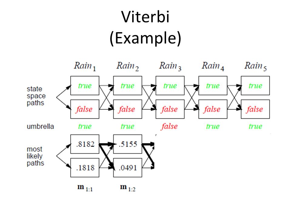
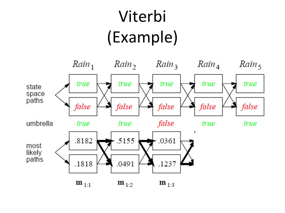
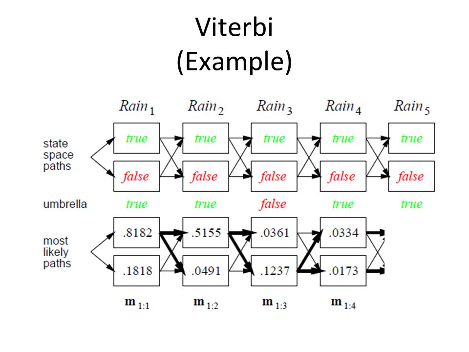
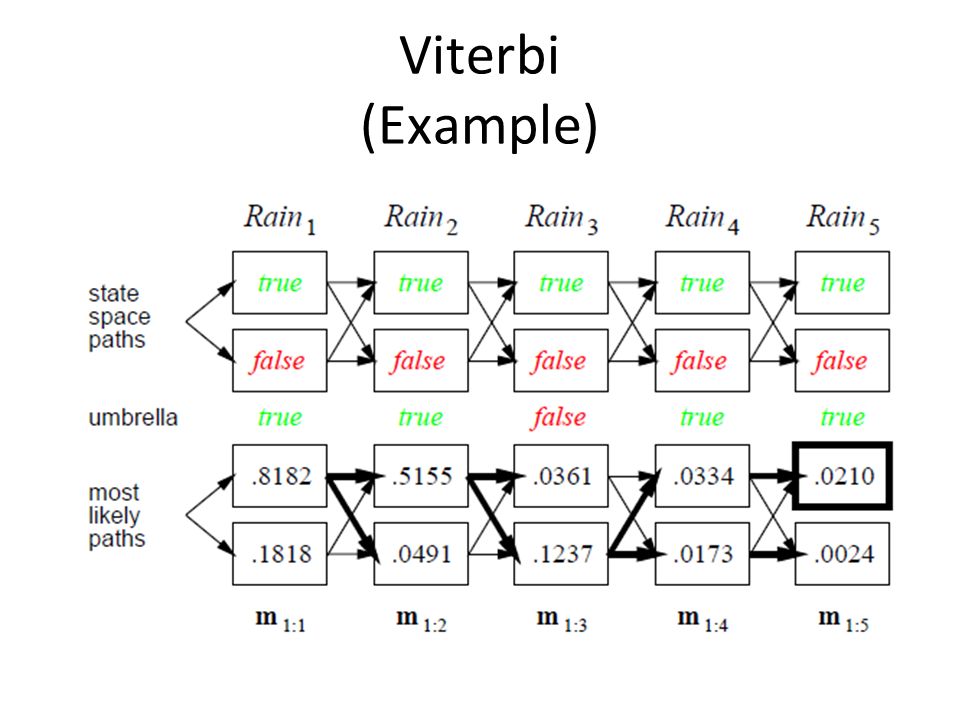
20. Most Likely Explanation Finding most likely path E t-1 E t+1 X t-1 XtXt X t+1 EtEt Called Viterbi

21. Viterbi (Example)

26. Today Time and uncertainty Inference: filtering, prediction, smoothing, MLE Hidden Markov Models (HMMs) –Model –Exact Reasoning Dynamic Bayesian Networks –Model –Exact Reasoning

27. Hidden Markov model (HMM) Y1Y1 Y3Y3 X1X1 X2X2 X3X3 Y2Y2 Phones/ words acoustic signal transition matrix Diagonal Matrix Sparse transition matrix ) sparse graph “True” state Noisy observations

28. Forwards algorithm for HMMs Predict: Update :

29. Message passing view of forwards algorithm Y t-1 Y t+1 X t-1 XtXt X t+1 YtYt  t|t-1 btbt b t+1

30. Forwards-backwards algorithm Y t-1 Y t+1 X t-1 XtXt X t+1 YtYt  t|t-1 tt btbt

31. If Have Time… Time and uncertainty Inference: filtering, prediction, smoothing Hidden Markov Models (HMMs) –Model –Exact Reasoning Dynamic Bayesian Networks –Model –Exact Reasoning

32. Dynamic Bayesian Network DBN is like a 2time-BN –Using the first order Markov assumptions Standard BN Time 0Time 1

33. Dynamic Bayesian Network Basic idea: –Copy state and evidence for each time step –Xt: set of unobservable (hidden) variables (e.g.: Pos, Vel) –Et: set of observable (evidence) variables (e.g.: Sens.A, Sens.B) Notice: Time is discrete

34. Example

35. Inference in DBN Unroll: Inference in the above BN Not efficient (depends on the sequence length)

36. DBN Representation: DelC TtTt LtLt CR t RHC t T t+1 L t+1 CR t+1 RHC t+1 f CR (L t, CR t, RHC t, CR t+1 ) f T (T t, T t+1 ) L CR RHC CR (t+1) CR (t+1) O T T 0.2 0.8 E T T 1.0 0.0 O F T 0.0 1.0 E F T 0.0 1.0 O T F 1.0 0.1 E T F 1.0 0.0 O F F 0.0 1.0 E F F 0.0 1.0 T T (t+1) T (t+1) T 0.91 0.09 F 0.0 1.0 RHM t RHM t+1 MtMt M t+1 f RHM (RHM t, RHM t+1 ) RHM R (t+1) R (t+1) T 1.0 0.0 F 0.0 1.0

37. Benefits of DBN Representation Pr (Rm t+1,M t+1,T t+1, L t+1,C t+1, Rc t+1 | Rm t,M t,T t, L t,C t, Rc t ) = f Rm (Rm t, Rm t+1 ) * f M (M t, M t+1 ) * f T (T t, T t+1 ) * f L (L t, L t+1 ) * f Cr (L t, Cr t, Rc t, Cr t+1 ) * f Rc (Rc t, Rc t+1 ) - Only few parameters vs. 25440 for matrix -Removes global exponential dependence s 1 s 2... s 160 s 1 0.9 0.05... 0.0 s 2 0.0 0.20... 0.1 s 160 0.1 0.0... 0.0...... TtTt LtLt CR t RHC t T t+1 L t+1 CR t+1 RHC t+1 RHM t RHM t+1 MtMt M t+1