1. CHAPTER 5 CMPT 310 Introduction to Artificial Intelligence Simon Fraser University Oliver Schulte Sequential Games and Adversarial Search

2. Environment Type Discussed In this Lecture Turn-taking: Semi-dynamic Deterministic and non-deterministic CMPT 310 - Blind Search 2 Fully Observable Multi-agent Sequential yes Discrete yes Game Tree Search yes no Continuous Action Games Game Matrices no yes

3. Sequential Games

4. Game Trees: Definition Every node is assigned to a player (turn). For every possible action of the player of the node, there is a child. The edge node  child is labelled with the action. The leaves of the tree specify the payoff for each player.

5. Hume’s Farmer Problem 1 2 2 2 0303 30301 H Not H H1 not H1 H2 Not H2 The payoffs for player 1 are listed at the top. Backward Induction: Look ahead and reason back.

6. The Story Two farmers need help with their harvest. Farmer 1 harvests before Farmer 2. If Farmer 1 asks Farmer 2 for help and receives it, Farmer 1 prefers not to reciprocate. If Farmer 1 does not reciprocate, Farmer 2 prefers not helping over helping. Both would rather help each other than harvest alone.

7. Trust on E-Bay SellerSeller 2 2 2 0303 30301 Send ItemNot Send Item send payment not send payment send payment

8. ADVERSARIAL SEARCH Zero-Sum Sequential Games

9. Adversarial Search Examine the problems that arise when we try to plan ahead in a world where other agents are planning against us. A good example is in board games. Adversarial games, while much studied in AI, are a small part of game theory in economics.

10. Typical AI assumptions Two agents whose actions alternate Utility values for each agent are the opposite of the other  creates the adversarial situation Fully observable environments In game theory terms: Zero-sum games of perfect information.

11. Search versus Games Search – no adversary  Solution is (heuristic) method for finding goal  Heuristic techniques can find optimal solution  Evaluation function: estimate of cost from start to goal through given node  Examples: path planning, scheduling activities Games – adversary  Solution is strategy (strategy specifies move for every possible opponent reply).  Optimality depends on opponent. Why?  Time limits force an approximate solution  Evaluation function: evaluate “goodness” of game position  Examples: chess, checkers, Othello, backgammon

12. Types of Games deterministicChance moves Perfect information Chess, checkers, go, othello Backgammon, monopoly Imperfect information (Initial Chance Moves) Bridge, SkatPoker, scrabble, blackjack on-line backgam mon on-line backgam mon on-line chess on-line chess

13. Zero-Sum Games of Perfect Information

14. Game Setup Two players: MAX and MIN MAX moves first and they take turns until the game is over  Winner gets award, loser gets penalty. Games as search:  Initial state: e.g. board configuration of chess  Successor function: list of (move,state) pairs specifying legal moves.  Terminal test: Is the game finished?  Utility function: Gives numerical value of terminal states. E.g. win (+1), lose (-1) and draw (0) in tic-tac-toe or chess

15. Size of search trees b = branching factor d = number of moves by both players Search tree is O(b d ) Chess  b ~ 35  D ~100 - search tree is ~ 10 154 (!!) - completely impractical to search this Game-playing emphasizes being able to make optimal decisions in a finite amount of time  Somewhat realistic as a model of a real-world agent  Even if games themselves are artificial

16. Partial Game Tree for Tic-Tac-Toe

17. Game tree (2-player, deterministic, turns) How do we search this tree to find the optimal move?

18. Minimax Search

19. Minimax strategy: Look ahead and reason backwards Find the optimal strategy for MAX assuming an infallible MIN opponent  Need to compute this all the down the tree  Game Tree Search Demo Game Tree Search Demo Assumption: Both players play optimally! Given a game tree, the optimal strategy can be determined by using the minimax value of each node. Zermelo 1912.

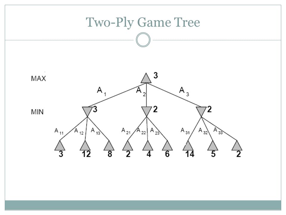
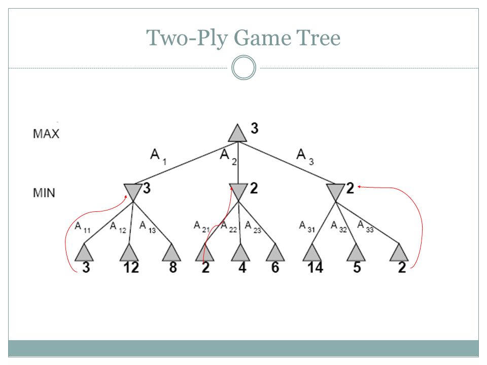
20. Two-Ply Game Tree

23. The minimax decision Minimax maximizes the utility for the worst-case outcome for max

24. What if MIN does not play optimally? Definition of optimal play for MAX assumes MIN plays optimally:  maximizes worst-case outcome for MAX But if MIN does not play optimally, MAX will do even better  Can prove this (Problem 6.2)

25. Pseudocode for Minimax Algorithm function MINIMAX-DECISION(state) returns an action inputs : state, current state in game v  MAX-VALUE(state) return the action in SUCCESSORS(state) with value v function MIN-VALUE(state) returns a utility value if TERMINAL-TEST(state) then return UTILITY(state) v  ∞ for a,s in SUCCESSORS(state) do v  MIN(v,MAX-VALUE(s)) return v function MAX-VALUE(state) returns a utility value if TERMINAL-TEST(state) then return UTILITY(state) v  -∞ for a,s in SUCCESSORS(state) do v  MAX(v,MIN-VALUE(s)) return v

26. Example of Algorithm Execution MAX to move

27. Minimax Algorithm Complete depth-first exploration of the game tree Assumptions:  Max depth = d, b legal moves at each point  E.g., Chess: d ~ 100, b ~35 CriterionMinimax TimeO(b d ) SpaceO(bd) 

28. Multiplayer games Games allow more than two players Single minimax values become vectors

29. Example A and B make simultaneous moves, illustrates minimax solutions. Can they do better than minimax? Can we make the space less complex? Pure strategy vs mix strategies Zero sum games: zero-sum describes a situation in which a participant's gain or loss is exactly balanced by the losses or gains of the other participant(s). If the total gains of the participants are added up, and the total losses are subtracted, they will sum to zero

30. Aspects of multiplayer games Previous slide (standard minimax analysis) assumes that each player operates to maximize only their own utility In practice, players make alliances  E.g, C strong, A and B both weak  May be best for A and B to attack C rather than each other If game is not zero-sum (i.e., utility(A) = - utility(B) then alliances can be useful even with 2 players  e.g., both cooperate to maximum the sum of the utilities

31. Alpha-Beta Pruning

32. Practical problem with minimax search Number of game states is exponential in the number of moves.  Solution: Do not examine every node => pruning  Remove branches that do not influence final decision Alpha-beta pruning: for each node, estimate interval of possible values.

33. Alpha-Beta Example [-∞, +∞] Initial Range of possible values Do DF-search until first leaf

34. Alpha-Beta Example (continued) [-∞,3] [-∞,+∞]

35. Alpha-Beta Example (continued) [-∞,3] [-∞,+∞]

36. Alpha-Beta Example (continued) [3,+∞] [3,3]

37. Alpha-Beta Example (continued) [-∞,2] [3,+∞] [3,3] This node is worse for MAX

38. Alpha-Beta Example (continued) [-∞,2] [3,14] [3,3][-∞,14],

39. Alpha-Beta Example (continued) [−∞,2] [3,5] [3,3][-∞,5],

40. Alpha-Beta Example (continued) [2,2] [−∞,2] [3,3]

41. Alpha-Beta Example (continued) [2,2] [-∞,2] [3,3]

42. Alpha-beta Algorithm Depth first search – only considers nodes along a single path at any time  = highest-value choice that we can guarantee for MAX so far in the current subtree.  = lowest-value choice that we can guarantee for MIN so far in the current subtree. update values of  and  during search and prunes remaining branches as soon as the value is known to be worse than the current  or  value for MAX or MIN. Alpha-beta Demo. Alpha-beta Demo

43. Exercise 3 41278 5 6 -which nodes can be pruned? MAX MIN MAX

44. Pseudocode for Alpha-Beta Algorithm function ALPHA-BETA-SEARCH(state) returns an action inputs: state, current state in game v  MAX-VALUE(state, - ∞, + ∞ ) return the action in SUCCESSORS(state) with value v

45. Pseudocode for Alpha-Beta Algorithm function ALPHA-BETA-SEARCH(state) returns an action inputs: state, current state in game v  MAX-VALUE(state, - ∞, + ∞ ) return the action in SUCCESSORS(state) with value v function MAX-VALUE(state, ,  ) returns a utility value if TERMINAL-TEST(state) then return UTILITY(state) v  - ∞ for a,s in SUCCESSORS(state) do v  MAX(v,MIN-VALUE(s, ,  )) if v ≥  then return v   MAX( ,v) return v

46. Alpha-Beta Analysis

47. Effectiveness of Alpha-Beta Search Worst-Case  branches are ordered so that no pruning takes place. In this case alpha-beta gives no improvement over exhaustive search Best-Case  each player’s best move is the left-most alternative (i.e., evaluated first)  in practice, performance is closer to best rather than worst-case In practice often get O(b (d/2) ) rather than O(b d )  this is the same as having a branching factor of √(b),  since (√b) d = b (d/2)  i.e., we have effectively gone from b to √b.  e.g., in chess go from b ~ 35 to b ~ 6  this permits much deeper search in the same amount of time  Typically twice as deep.

48. Final Comments about Alpha-Beta Pruning Pruning does not affect final results Entire subtrees can be pruned. Good move ordering improves effectiveness of pruning Repeated states are again possible.  Store them in memory = transposition table

49. Game Playing Practice

50. Practical Implementation How do we make these ideas practical in real game trees? Standard approach: evaluation function cutoff test: where do we stop descending the tree Return evaluation of best position when search is cut off.

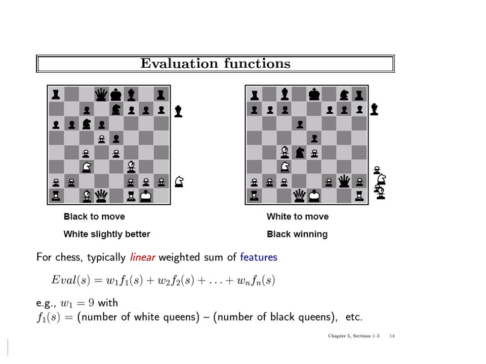
51. Static (Heuristic) Evaluation Functions An Evaluation Function:  estimates how good the current board configuration is for a player.  Typically, one figures how good it is for the player, and how good it is for the opponent, and subtracts the opponents score from the players  Othello: Number of white pieces - Number of black pieces  Chess: Value of all white pieces - Value of all black pieces Typical values from -infinity (loss) to +infinity (win) or [-1, +1]. If the board evaluation is X for a player, it’s -X for the opponent. Many clever ideas about how to use the evaluation function.  e.g. null move heuristic: let opponent move twice. Example:  Evaluating chess boards,  Checkers  Tic-tac-toe

53. Iterative (Progressive) Deepening In real games, there is usually a time limit T on making a move. How do we take this into account?  using alpha-beta we cannot use “partial” results with any confidence unless the full breadth of the tree has been searched  So, we could be conservative and set a conservative depth-limit which guarantees that we will find a move in time < T  disadvantage is that we may finish early, could do more search In practice, iterative deepening search (IDS) is used  IDS runs depth-first search with an increasing depth-limit  when the clock runs out we use the solution found at the previous depth limit

54. Heuristics and Game Tree Search The Horizon Effect  sometimes there’s a major “effect” (such as a piece being captured) which is just “below” the depth to which the tree has been expanded the computer cannot see that this major event could happen it has a “limited horizon”

55. The State of Play Checkers:  Chinook ended 40-year-reign of human world champion Marion Tinsley in 1994. Chess:  Deep Blue defeated human world champion Garry Kasparov in a six-game match in 1997. Othello:  human champions refuse to compete against computers: they are too good. Go:  human champions refuse to compete against computers: they are too bad b > 300 (!) See (e.g.) http://www.cs.ualberta.ca/~games/ for more information http://www.cs.ualberta.ca/~games/

57. Deep Blue 1957: Herbert Simon  “within 10 years a computer will beat the world chess champion” 1997: Deep Blue beats Kasparov Parallel machine with 30 processors for “software” and 480 VLSI processors for “hardware search” Searched 126 million nodes per second on average  Generated up to 30 billion positions per move  Reached depth 14 routinely Uses iterative-deepening alpha-beta search with transpositioning  Can explore beyond depth-limit for interesting moves

58. Chance Games. Backgammon your element of chance

59. Expected Minimax Interleave chance nodes with min/max nodes Again, the tree is constructed bottom-up

60. Summary: Solving Games Zero-sumNon zero-sum Perfect InformationMinimax, alpha-betaBackward induction, retrograde analysis Imperfect InformationProbabilistic minimaxNash equilibrium

61. Summary Game playing can be effectively modeled as a search problem Game trees represent alternate computer/opponent moves Evaluation functions estimate the quality of a given board configuration for the Max player. Minimax is a procedure which chooses moves by assuming that the opponent will always choose the move which is best for them Alpha-Beta is a procedure which can prune large parts of the search tree and allow search to go deeper For many well-known games, computer algorithms based on heuristic search match or out-perform human world experts.

62. Single Agent vs. 2-Players Every single agent problem can be considered as a special case of a 2-player game. How? 1. Make one of the players the Environment, with a constant utility function (e.g., always 0). 1. The Environment acts but does not care. 2. An adversarial Environment, with utility function the negative of agent’s utility. 1. In minimization, Environment’s utility is player’s costs. 2. Worst-Case Analysis. 3. E.g., program correctness: no matter what input user gives, program gives correct answer. So agent design is a subfield of game theory.

63. Single Agent Design = Game Theory Von Neumann-Morgenstern Games Decision Theory = 2-player game, 1st player the “agent”, 2 nd player “environment/nature” (with constant or adversarial utility function) Markov Decision Processes Planning Problems From General To Special Case

64. Example: And-Or Trees If an agent’s actions have nondeterministic effects, we can model worst-case analysis as a zero-sum game where the environment chooses the effects of an agent’s actions. Minimax Search ≈ And-Or Search. Example: The Erratic Vacuum Cleaner.  When applied to dirty square, vacuum cleans it and sometimes adjacent square too.  When applied to clean square, sometimes vacuum makes it dirty.  Reflex agent: same action for same location, dirt status.

65. And-Or Tree for the Erratic Vacuum The agent “moves” at labelled OR nodes. The environment “moves” at unlabelled AND nodes. The agent wins if it reaches a goal state. The environment “wins” if the agent goes into a loop.

66. Summary Game Theory is a very general, highly developed framework for multi-agent interactions. Deep results about equivalences of various environment types. See Chapter 17 for more details.