Download presentation
Presentation is loading. Please wait.

1
Machine Learning Expectation Maximization and Gaussian Mixtures CSE 473 Chapter 20.3

2
Feedback in Learning Supervised learning: correct answers for each example Unsupervised learning: correct answers not given Reinforcement learning: occasional rewards

3
The problem of finding labels for unlabeled data So far we have solved “supervised” classification problems where a teacher told us the label of each example. In nature, items often do not come with labels. How can we learn labels without a teacher? Unlabeled data -10-8-6-4-2 -6 -4 -2 0 2 4 6 Labeled data From Shadmehr & Diedrichsen

4
Example: image segmentation Identify pixels that are white matter, gray matter, or outside of the brain. 0.20.40.60.81 250 500 750 1000 1250 1500 Outside the brain Gray matter White matter Pixel value (normalized) From Shadmehr & Diedrichsen
 From Shadmehr & Diedrichsen.")
5
Raw Proximity Sensor Data Measured distances for expected distance of 300 cm. SonarLaser

7
Gaussians -- Univariate Multivariate

8
© D. Weld and D. Fox 8 Fitting a Gaussian PDF to Data Poor fitGood fit From Russell

9
© D. Weld and D. Fox 9 Fitting a Gaussian PDF to Data Suppose y = y 1,…,y n,…,y N is a set of N data values Given a Gaussian PDF p with mean and variance , define: How do we choose and to maximise this probability? From Russell

10
© D. Weld and D. Fox 10 Maximum Likelihood Estimation Define the best fitting Gaussian to be the one such that p(y| , ) is maximised. Terminology: p(y| , ), thought of as a function of y is the probability (density) of y p(y| , ), thought of as a function of , is the likelihood of , Maximizing p(y| , ) with respect to , is called Maximum Likelihood (ML) estimation of , From Russell
 is maximised. Terminology: p(y| , ), thought of as a function of y is the probability (density) of y p(y| , ), thought of as a function of , is the likelihood of , Maximizing p(y| , ) with respect to , is called Maximum Likelihood (ML) estimation of , From Russell.")
11
© D. Weld and D. Fox 11 ML estimation of , Intuitively: The maximum likelihood estimate of should be the average value of y 1,…,y N, (the sample mean) The maximum likelihood estimate of should be the variance of y 1,…,y N. (the sample variance) This turns out to be true: p(y| , ) is maximised by setting: From Russell
 The maximum likelihood estimate of should be the variance of y 1,…,y N. (the sample variance) This turns out to be true: p(y| , ) is maximised by setting: From Russell.")
12
© D. Weld and D. Fox 12

13
© D. Weld and D. Fox 13

14
© D. Weld and D. Fox 14

15
If our data is not labeled, we can hypothesize that: 1.There are exactly m classes in the data: 2.Each class y occurs with a specific frequency: 3.Examples of class y are governed by a specific distribution: According to our hypothesis, each example x (i) must have been generated from a specific “mixture” distribution: We might hypothesize that the distributions are Gaussian: Mixtures Parameters of the distributions Mixing proportionsNormal distribution
 must have been generated from a specific mixture distribution: We might hypothesize that the distributions are Gaussian: Mixtures Parameters of the distributions Mixing proportionsNormal distribution")
16
Hidden variable Measured variable y Py Graphical Representation of Gaussian Mixtures

17
Learning of mixture models

18
Learning Mixtures from Data Consider fixed K = 2 e.g., Unknown parameters = { 1 , 1, 2 , 2, } Given data D = {x 1,…….x N }, we want to find the parameters that “best fit” the data

19
Early Attempts Weldon’s data, 1893 - n=1000 crabs from Bay of Naples - Ratio of forehead to body length - Suspected existence of 2 separate species

20
Early Attempts Karl Pearson, 1894: - JRSS paper - proposed a mixture of 2 Gaussians - 5 parameters = { 1 , 1, 2 , 2, } - parameter estimation -> method of moments - involved solution of 9th order equations! ( see Chapter 10, Stigler (1986), The History of Statistics )
, The History of Statistics ).")
21
“The solution of an equation of the ninth degree, where almost all powers, to the ninth, of the unknown quantity are existing, is, however, a very laborious task. Mr. Pearson has indeed possessed the energy to perform his heroic task…. But I fear he will have few successors…..” Charlier (1906)
.")
22
Maximum Likelihood Principle Fisher, 1922 assume a probabilistic model likelihood = p(data | parameters, model) find the parameters that make the data most likely
 find the parameters that make the data most likely")
23
1977: The EM Algorithm Dempster, Laird, and Rubin General framework for likelihood-based parameter estimation with missing data start with initial guesses of parameters E-step: estimate memberships given params M-step: estimate params given memberships Repeat until convergence Converges to a (local) maximum of likelihood E-step and M-step are often computationally simple Generalizes to maximum a posteriori (with priors)
 maximum of likelihood E-step and M-step are often computationally simple Generalizes to maximum a posteriori (with priors)")
24
© D. Weld and D. Fox 24 EM for Mixture of Gaussians E-step: Compute probability that point x j was generated by component i: M-step: Compute new mean, covariance, and component weights:

33
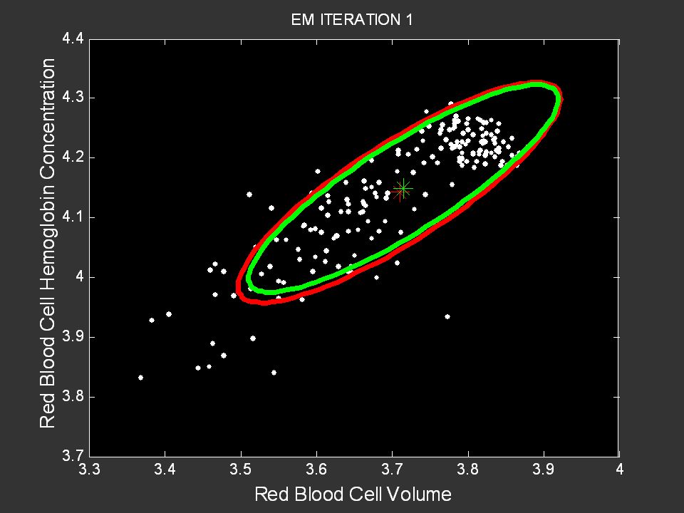
Anemia Group Control Group

34
Mixture Density How can we determine the model parameters?

35
Raw Sensor Data Measured distances for expected distance of 300 cm. SonarLaser

36
Approximation Results Sonar Laser 300cm400cm

37
© Daniel S. Weld 37 Hidden Variables But we can’t observe the disease variable Can’t we learn without it?

38
© Daniel S. Weld 38 We –could- But we’d get a fully-connected network With 708 parameters (vs. 78) Much harder to learn!
 Much harder to learn!.")
39
© Daniel S. Weld 39 Chicken & Egg Problem If we knew that a training instance (patient) had the disease… It would be easy to learn P(symptom | disease) But we can’t observe disease, so we don’t. If we knew params, e.g. P(symptom | disease) then it’d be easy to estimate if the patient had the disease. But we don’t know these parameters.
 had the disease… It would be easy to learn P(symptom | disease) But we can’t observe disease, so we don’t. If we knew params, e.g. P(symptom | disease) then it’d be easy to estimate if the patient had the disease. But we don’t know these parameters..")
40
© Daniel S. Weld 40 Expectation Maximization (EM) (high-level version) Pretend we do know the parameters Initialize randomly [E step] Compute probability of instance having each possible value of the hidden variable [M step] Treating each instance as fractionally having both values compute the new parameter values Iterate until convergence!
 (high-level version) Pretend we do know the parameters Initialize randomly [E step] Compute probability of instance having each possible value of the hidden variable [M step] Treating each instance as fractionally having both values compute the new parameter values Iterate until convergence!.")
Similar presentations


 and the class- conditional probabilities P(x|wi)>")


. Goal : assume the.>")

 Dealing with Indefinite Representations in Pattern Recognition.>")


