1. Report due: March 31, electronically submit, pdf format. Find a computational research article (5 pages or more) from one of the following journals: Bioinformatics BMC Bioinformatics Genome Research Journal of Proteome Research Nucleic Acids Research The article needs to be published after 1/1/2015. Write a report based on the study of the paper, and its citations.

2. Report due: March 31, electronically submit, pdf format. Requirements: 8 Pages, 1’’ margin, 1.5 line spacing not including figures/tables. Figures/tables need to be attached at the end of the document. Include (but not limited to) the following components: Background and significance of the work. What’s the technical improvement of the work over previous works? What could have been done better? If you were the authors, what’s your next step to extend this work?

3. Networks in Bioinformatics General Characteristics Directed Acyclic Graph and Gene Ontology Defining distances on DAGs Network and expression data Testing on an existing network Reverse engineering of networks

4. Network / Graph A network is a set of vertices connected by edges. undirected edges  “undirected network” directed edges  “directed network”. Vertex-level characteristic: The number of connections to a vertex : “degree” Incoming edges  “in-degree” k i Outgoing edges  “out-degree” k o k=k i +k o kiki koko Evolution of networks. S.N. Dorogovtsev, J.F.F. Mendes

5. Network Network-level characteristics: Number of vertices: N Number of edges: L Number of loops: I For an undirected network: I=L-N+1 Degree: The distribution of vertex degrees

6. Network Distribution of shortest path: ℓ μν is the shortest path between nodes u and v The mean value is called the “diameter” of the network Clustering coefficient: For each vertex, the fraction of existing connections between nearest neighbors of the vertex: C (μ) ≡ y (μ) /[z (μ) (z (μ) − 1)/2], z (μ) : Number of neighboring vertices y (μ) : Number of edges between the neighboring vertices Clustering coefficient C is the mean of C (μ)

7. Scale-free Network Scale-free network: The degree distribution follows the power law: Few nodes are of high degree, while most nodes are of low degree. Contrast: random edge generation yields Poisson distribution.

8. Scale-free Network Nature 406(6794):378. Quote from the figure legend: Both networks contain 130 nodes and 215 links. Red, the five nodes with the highest number of links; green, their first neighbours.

9. A large number of real-world networks, including biological networks are found to have power law degree distribution. Some nodes serve as “hubs”. This makes sense for WWW, social networks, and for biological networks, where controllers like the transcription factors are well known. Scale-free networks are “ultra small-world” – most nodes can reach one another in a few steps. These networks exhibit “high tolerance to random perturbations but are sensitive to targeted attack on the highly connected nodes”.

10. One way to generate a network with such distribution is the “rich get richer” model by Barabási and Albert (1999): Initiate a network, with degree ≥ 1 for each node; Add new node to the network, linking to existing nodes with probabilities:, where k i is the degree of the node. Higher-degree nodes are more likely to gain new connections. Scale-free Network

11. The protein-protein interaction network is a scale-free network. S. Wuchty, E. Ravasz and A.-L. Baraba¶si: The Architecture of Biological Networks Scale-free Network

12. Bioinformaticians’ interest in network Characterizing the structure of biological networks, and find functional and evolutionary implications. (a) Ashbya gossypii ATCC 10895 (b) Burkholderia sp. (c) human Scientific Reports 5, 15567 (2015) “The compounds that have multiple pathways to the core compounds are less likely to cause diseases than the compounds without multiple pathways.”

13. Bioinformaticians’ interest in network Characterizing the behavior of network nodes/subnetworks on an existing network. BMC Genomics,15:314

14. Bioinformaticians’ interest in network Reverse engineering of networks based on observations of gene expression behavior – inference of regulatory relations. Current Genomics, 2015, 16, 3-22

15. Bioinformaticians’ interest in network Disease etiology

16. Bioinformaticians’ interest in network Disease etiology

17. Testing on the network Goal: Utilize existing network to aid biomarker selection (“network marker”) disease mechanism finding predictive model building Data: A network between biological units Signal transduction network Genetic interaction network Protein-protein interaction network TF regulatory network …… Behavior of nodes Expression data Knock-out data …...

18. Testing on the network An example of machine- learning approach. Mol Syst Biol. 2007; 3: 140.

19. Testing on the network Mol Syst Biol. 2007; 3: 140. Network markers: Diamond – univariate significant

20. Testing on the network Ann. Appl. Stat. (Epub ahead of print) Example: A Bayesian framework  Univariate test of all genes  Transform p-values to normal quantiles  Assume a gene is either “1” (disease related) or “0” (unrelated)  Use a network-based mixture model – neighboring genes are more likely to share status

21. Reverse engineering of networks from microarray data Goal: infer genetic regulation network structure from microarray data Key assumption: The mRNA level measured by microarray truly reflects the activity of the regulator Sadly this is only true for ~20% of the regulators Methods incorporating more data/knowledge are developed

22. Reverse engineering of networks from microarray data Margolin & Califano, Ann N Y Acad Sci. 2007,1115:51. Hesselberth et al. Genome Biology. 2006,7:R30.

23. Reverse engineering of networks from microarray data Correlation Partial correlation (Gaussian graphical models) Expression data alone Expression data + other information Known transcription factor targets ChIP-chip and ChIP-seq Known interactions/pathways … Mutual information Bayesian network

24. Reverse engineering of networks from microarray data Margolin & Califano, Ann N Y Acad Sci. 2007,1115:51. Differentiating mechanisms of co-regulation based on expression data alone is a daunting task.

25. Network for knowledge representation Directed Acyclic Graph (DAG) Directed graph with no directed loops, i.e. from any node, no route to come back to the same node. The structure leads to partial ordering of the nodes: If an edge i  j exists, node i is at higher level than node j.

26. Organize knowledge about genes in a directed acyclic graph. The lower the level, the more detailed knowledge. Each gene is annotated to the terms, reflecting people’s knowledge about it. The Gene-Ontology knowledge-base

27. Similar thinking has been used on the tree of life and other areas Mol. BioSyst., 2014, 10, 86-92

28. Here’s how people’s knowledge about the gene ACE2 is summarized using the database. Based on these papers: The Gene-Ontology knowledge-base

29. Gene ontology and high-throughput data Gene ontology was necessitated by high-throughput data --- when thousands of genes are measured simultaneously, people must be able to combine the results with existing knowledge in a computationally efficient way.

30. Gene ontology and high-throughput data Two general types of considerations:  Does a GO term have first-order association with the clinical outcome?  Does the GO term change its interactions with other functional units in response to the clinical factor?

31. Gene ontology and high-throughput data How to deal with dependency between (neighboring) GO terms ? General strategies: Treat all GO terms as independent units, test for significant changes one-by-one, and let biologists remove the redundant information. Using the GO structure to remove redundant terms, and only test a small informative subset of all GO terms. Test for independence conditioned on the results of descendant nodes.

32. Gene ontology and high-throughput data Given a GO term, how to find whether it is up- or down- regulated in association with disease is an active research area. We list a few examples here. Difficulty: Within each GO term, a number of genes exist. These genes in fact operate in a network fashion in the cell. Competitions and feed back loops are common. The genes in one GO term don’t change in one direction. In association with a disease, some are up-regulated, some are suppressed, and some don’t change.

33. Gene ontology and high-throughput data GO term: positive regulation of I-kappaB kinase/NF-kappaB cascade Disease: Oral cancer metastasis

34. Gene ontology and high-throughput data Cutoff-based methods: General Idea: Test significance gene-by-gene. Select a threshold level, divide all genes into two groups: differentially expressed and non-differentially expressed. For each GO term, test the hypothesis that the differentially expressed genes are drawn from the pool of all genes independent of the GO term. Hypergeometric Binomial Chi-square test … … The arbitrary threshold has substantial impact on the results.

35. Gene ontology and high-throughput data Cutoff-free methods: Try to avoid the use of arbitrary threshold. Usually use permutation tests to find significance. This ensures the correlation structure between the genes are preserved. With group of genes to analyze, the hypothesis becomes complicated. Different method may use different assumptions and test for different hypotheses.

36. Gene ontology and high-throughput data JOURNAL OF COMPUTATIONAL BIOLOGY. 13:798. Comparing the p-value （ or correlation, or other statistics) distributions from one GO term to the overall distribution:  Kolmogorov–Smirnov goodness-of-fit test statistic for comparing two distributions  Anderson–Darling test statistic for testing for a uniform distribution  Wilcoxon rank-sum test statistic

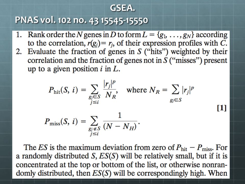
37. GSEA. PNAS vol. 102 no. 43 15545-15550

39. The competitive null hypothesis: genes in the gene set are not more associated with the phenotype than genes outside the gene set. The self-contained null hypothesis: no genes in the gene set are associated with the phenotype. Gene ontology and high-throughput data

40. GSDCA. Single gene set gene set pairs

41. GSDCA.