Download presentation
Presentation is loading. Please wait.

1
DATA ANALYSIS AND MODEL BUILDING LECTURE 9 Prof. Roland Craigwell Department of Economics University of the West Indies Cave Hill Campus and Rebecca Gookool Department of Economics University of the West Indies St. Augustine Campus

2
Multiple Linear Regression Multiple Linear Regression

3
Linear Regression

4
Properties of the Hat matrix

5
Variance-Covariance Matrices

6
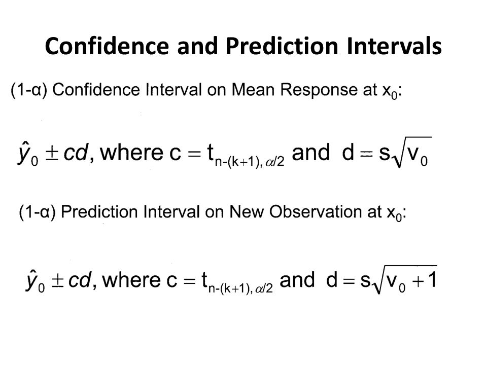
Confidence and Prediction Intervals

8
Sums of Squares

9
Overall Significance Test

10
Scatter plot Matrix of the Air Data Set in S-Plus pairs(air)
")
11
Polynomial Models y=β 0 + β 1 x+ β 2 x 2 …+ β k x k Problems: Powers of x tend to be large in magnitude Powers of x tend to be highly correlated Solutions: Centering and scaling of x variables Orthogonal polynomials

12
Plot of mpg vs. weight for 74 autos

13
Orthogonal Polynomials Generation is similar to Gram-Schmidt orthogonalization (see Strang, Linear Algebra) Resulting vectors are orthonormal X’X=I Hence (X’X)-1= I and coefficients = (X’X)-1X’y = X’y Addition of higher degree term does not affect coefficients for lower degree terms Correlation of coefficients = I SE of coefficients = s = sqrt(MSE)
 Resulting vectors are orthonormal X’X=I Hence (X’X)-1= I and coefficients = (X’X)-1X’y = X’y Addition of higher degree term does not affect coefficients for lower degree terms Correlation of coefficients = I SE of coefficients = s = sqrt(MSE)")
14
Plot of mpg by weight with fitted regression

15
Indicator Variables Sometimes we might want to fit a model with a categorical variable as a predictor. For instance, automobile price as a function of where the car is made (Germany, Japan, USA). If there are c categories, we need c-1 indicator (0,1) variables as predictors. For instance j=1 if car is made in Japan, 0 otherwise, u=1 if car is made in USA, 0 otherwise. If there are just 2 categories and no other predictors, we could just do a t-test for difference in means.
. If there are c categories, we need c-1 indicator (0,1) variables as predictors. For instance j=1 if car is made in Japan, 0 otherwise, u=1 if car is made in USA, 0 otherwise. If there are just 2 categories and no other predictors, we could just do a t-test for difference in means..")
16
Box plots of price by country

17
Histogram of automobile prices

18
Histogram of log of automobile prices

19
Regression Diagnostics Goal: identify remarkable observations and unremarkable predictors. Problems with observations: Outliers Influential observations Problems with predictors: A predictor may not add much to model. A predictor may be too similar to another predictor (collinearity). Predictors may have been left out.
. Predictors may have been left out..")
20
Plot of standardized residuals vs. fitted values for air dataset

21
Plot of residual vs. fit for air data set with all interaction terms

22
Plot of residual vs. fit for air model with x3*x4 interaction

23
Remarkable Observations

24
Plot of standardized residual vs. observation number for air dataset

25
Hat matrix diagonals

26
Plot of wind vs. ozone

27
Cook’s Distance

28
Plot of ozone vs. wind including fitted regression lines with and without observation 30 (simple linear regression)
.")
29
Remedies for Outliers Nothing? Data Transformation? Remove outliers? Robust Regression –weighted least squares: b=(X’WX)-1X’Wy Minimize median absolute deviation
-1X’Wy Minimize median absolute deviation.")
30
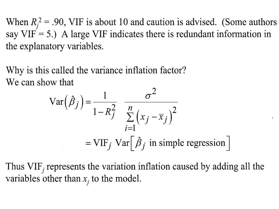
Collinearity High correlation among the predictors can cause problems with least squares estimates (wrong signs, low t-values, unexpected results). If predictors are centered and scaled to unit length, then X’X is the correlation matrix. Diagonal elements of inverse of correlation matrix are called VIF’s (variance inflation factors). is the coefficient of determination for the regression of the jth predictor on the remaining predictors
. is the coefficient of determination for the regression of the jth predictor on the remaining predictors.")
32
Remedies for collinearity 1.Identify and eliminate redundant variables (large literature on this). 2.Modified regression techniques a.ridge regression, b=(X’X+cI)-1X’y 3.Regress on orthogonal linear combinations of the explanatory variables a.principal components regression 4.Careful variable selection
-1X’y 3.Regress on orthogonal linear combinations of the explanatory variables a.principal components regression 4.Careful variable selection.")
33
Correlation and inverse of correlation matrix for air data set.

34
Correlation and inverse of correlation matrix for mpg data set

35
Variable Selection We want a parsimonious model – as few variables as possible to still provide reasonable accuracy in predicting y. Some variables may not contribute much to the model. SSE never will increase if add more variables to model, however MSE=SSE/(n-k-1) may. Minimum MSE is one possible optimality criterion. However, must fit all possible subsets (2kof them) and find one with minimum MSE.
 may. Minimum MSE is one possible optimality criterion. However, must fit all possible subsets (2kof them) and find one with minimum MSE..")
36
Backward Elimination 1.Fit the full model (with all candidate predictors). 2.If P-values for all coefficients < α then stop. 3.Delete predictor with highest P-value 4.Refit the model 5.Go to Step 2.

37
The end

Similar presentations


 2004 Brooks/Cole, a division of Thomson Learning, Inc. Chapter 13 Nonlinear and Multiple Regression.>")


 Review>")


