2. Some Topics in B Physics Y ing L i Y onsei U niversity, K orea Y antai U nviersity, C hina

3.  Introduction  B physics and CP violation  Factorization Approach  QCDF Vs PQCD  B  VV  No Summary

4.  Introduction  QCD and the SM have promoted the development of the particle physics remarkably, however, they should been tested in more experiments accurately.  The SM is regarded as an effective theory of some high- energy physics, and B physics is a good place for searching of new physics  It have been proved that B physics is also a good place in studying CP violation. And CPV has been measured in B factories, but its mechanism is still unknown.

5.  CLEO (The energy has been dropped)  Belle @ KEK and BaBar @ SLAC  Tavatron @ Fermi  LHC-b  Super-B......  Experimental Status

6.  Quark mixing and CKM

7.  Unitary triangle and CKM Phase

8.  Measurement of CKM Phase

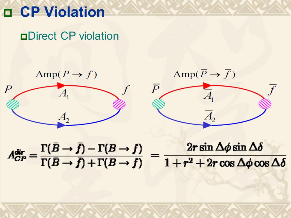
10.  CP Violation  Direct CP violation

11.  Oscillation CP Violation

12.  Mixing CP Violation

13.  Effective theory

14. Effective Vertex

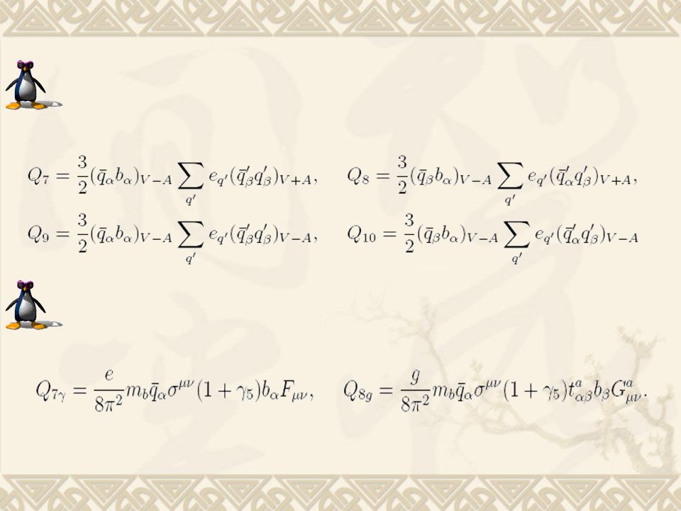
15. Penguins    (1-  5 ) : V-A   (1+  5 ): V+A At O(  s ) or O(  ), there are also penguin diagrams  QCD penguin: g EW penguin: g replaced by , Z 2 Color flows: 2T a ij T a kl = -  ij  kl /N c +  il  kj bs b q q s q q

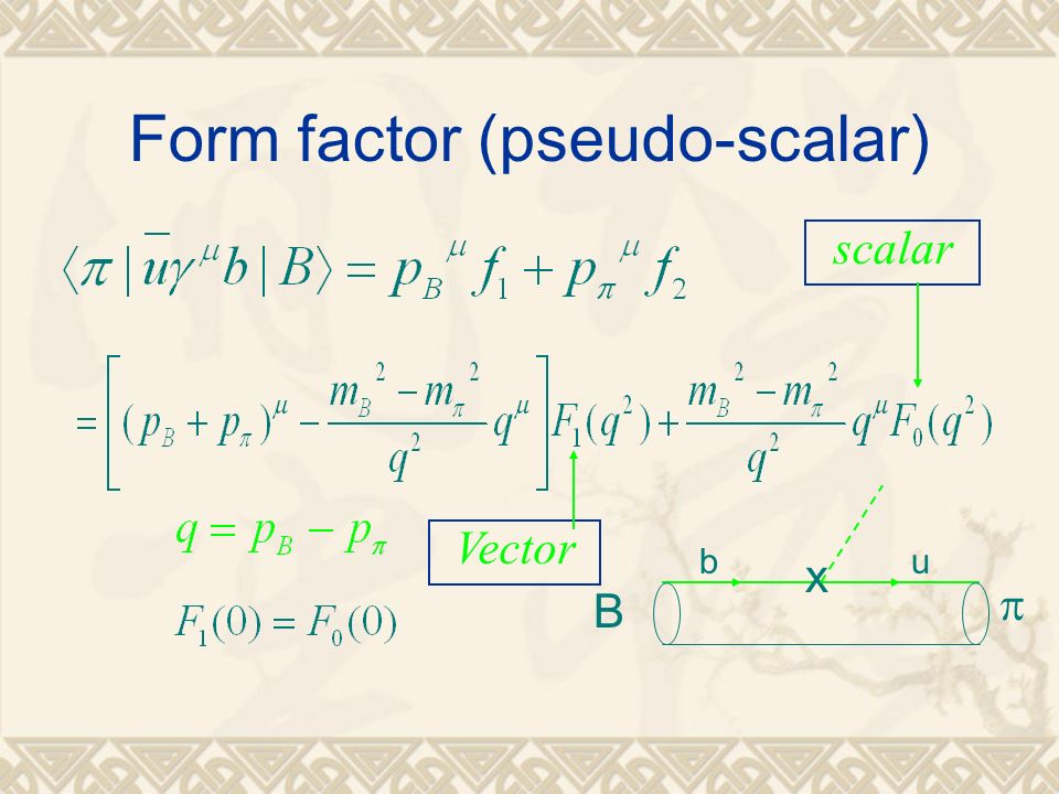
19. Form factor (pseudo-scalar) B  x bu Vector scalar

20. Vector meson  Vector current  Axial-vector current

21.  Research of B meson decay  Naive Factorization (B.S.W)  Generalized Factorization (Ali, C-D Lu, H-Y Cheng)  BBNS-Factorization (BBNS, Du, Yang,…)  Perturbative QCD approach (H-N Li, Sanda, Lu, ….)  Soft-collinear effective theory (SCET) (Stewart, Bauer, Pirjol,…)

22. Factorization vs. factorization  Factorization in “naïve factorization” means breaking a decay amplitude into decay constant and form factor.  Factorization in “factorization theorem” means separation of soft and hard dynamics in decay modes.  After 2000, factorization approach to exclusive B decays changed from 1st sense to 2nd.

23. Decay amplitudes a 1, a 2 : universal parameters Class 1: Color-allowed Class 2: Color-suppressed

24. B  D  (x10 –4 ) Decay modeTheoryex D* +  – 2927.6±2.1 D+ –D+ – 3030±4 D* 0  0 1.01.7±0.5 D0 0D0 0 0.72.9±0.5 D *0  + 4846±4 D0 +D0 + 4853±5 M. Neubert, B.Stech, hep- ph/9705292 a 1 =1.08 a 2 =0.21

25. B→ π + π – π + π + W u B 0 π – (D – ) B π – (D – ) dd C 2 ~ 1 > C 1 /3 ~ – 0.2/3

26. B→ππ,πρ,πω π (  ) W b u T ∝ V ub V ud * B π d π (  ) W b t P ∝ V tb V td * B π O 3,O 4,O 5,O 6 O 1,O 2

27. B→ππ 3 3

28. Disadvantage  We can not predict the contribution from NF  Form factors are borrowed from other theory  In this approach, the annihilation diagrams can not be calculated  There is no strong phase (or small phase), can not predict the cp violation  scale dependence  Large final states interaction

29. QCDF  The plausible proposal was realized by BBNS  Form factor F, DAs  absorb IR divergences. T are the hard kernels. (P 1 ) (P 2 )

30. Hard kernels I  T I comes from vertex corrections  The first 4 diagrams are IR finite, extract the  dependence of the matrix element.  q=P 1 +xP 2 is well-defined, q 2 =xm B 2  IR divergent, absorbed into F Magnetic penguin O 8g q 1 x g

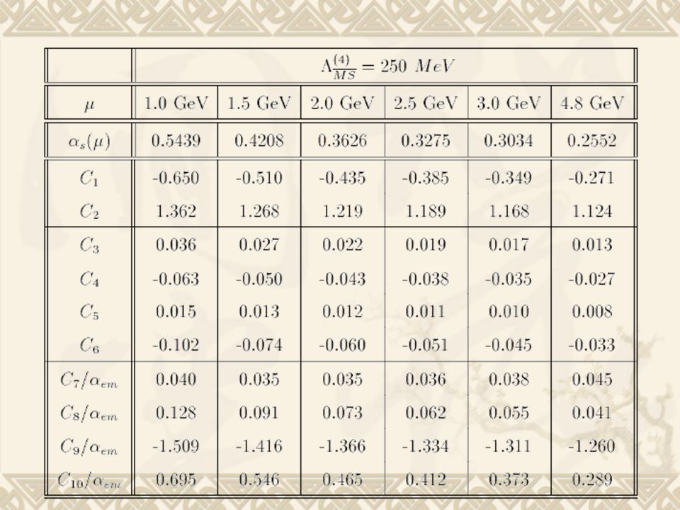
31. Wilson coefficients  Define the standard combinations,  Adding vertex corrections

32. Scale independence Dotted: no VC; solid: Re part with VC; dashed: Im part with VC

33. Scale independence The  dependence of most a i is moderated. That of a 6, a 8 is not. It will be moderated by combining m 0 (  ).

34. Hard kernels II  T II comes from spectator diagrams  Nonfactorizable contribution to FA and strong phase from the BSS mechanism can be computed.  QCDF=FA + subleading corrections, respects the factorization limit.  QCDF is a breakthrough!

35. End-point singularity  Beyond leading power (twist), end-point singularity appears at twist-3 for spectator amplitudes.  Also in annihilation amplitudes  parameterization Phase parameters are arbitrary.

36. Predictive power  For QCDF to have a predictive power, it is better that subleading (singular) corrections, especially annihilation, are small.  Predictions for direct CP asymmetries from QCDF are then small, close to those from FA.  Large theoretical uncertainty from the free parameters.

37. Power counting in QCDF Annihilation is power suppressed Due to helicity conservation

38. B   ,  K branching ratios For Tree- dominated modes, close to FA For penguin- dominated modes, larger than FA by a factor 2 due to O 8g.

39. B  ,  K direct CP asy. In FA, direct CP asy.» 0 B-BB+BB-BB+B

40. Direct CP asy. data Opposite to QCDF predictions!! To explain data, subleading corrections must be large, Which, however, can not be reliably computed in QCDF.

41. Introduction to PQCD Approach  A ~ ∫d 4 k 1 d 4 k 2 d 4 k 3 Tr [ C(t)  B (k 1 )  1 (k 2 )  2 (k 3 ) H(k 1,k 2,k 3,t) ] exp{–S(t)}   (k) is wave function in the light cone, which is universal.  C(t) : Wilson coefficients of corresponding four quark operators  exp{-S(t)} are Sudukov form factor (double log resummation) ， which relate the long distance contribution and short one. And the long distance effects have been suppressed.  H(k 1,k 2,k 3,t) is six quark interaction, and it can be calculated perturbatively, and it is process depended.

42.  Sudakov form factor

43.  Wave function

44.  Summary

45. QCDF  Form factor is a parameter  Wave function is a parameter  By Ignoring the transverse momentum ， there is a end-point singularity PQCD  Form factor can be calculated directly.  Wave function is a parameter  Keep transverse momentum, the sudakov form factor can kill the endpoint singularity

46. QCDF  Can not calculate the non- factorizable diagram and annihilation diagram effectively  non-factorizable diagram belong to α s correction  The Wilson coefficients have been at NNLO PQCD  Can calculate the non- factorizable diagram and annihilation diagram effectively  non-factorizable diagram belong to α s correction, as well as factorizable diagrams  The Wilson coefficients have been calculated in NLO partly.

47. Spectator Diagram

48. Annihilation Diagrams

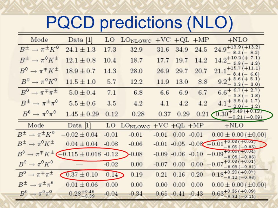
51. PQCD predictions (NLO)

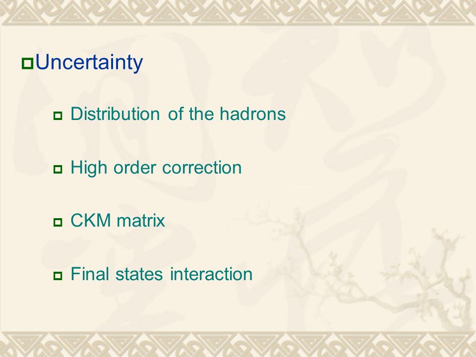
54.  Uncertainty  Distribution of the hadrons  High order correction  CKM matrix  Final states interaction

55. Color-allowed Color-suppressed factorizable Wilson coeff SCET factorization formula for B  M 1 M 2

56. Summary  QCDF, PQCD, SCET go beyond FA.  They have different assumptions, whose verification or falsification may not be easy.  They all have interesting phenomenological applications.  Huge uncertainty from QCDF is annoying. Input from time-like form factor for annihilation?  NLO correction in PQCD needs to be checked.  SCET should be applied to explore heavy quark decay dynamics more.

57.  B  VV

58. B  VV

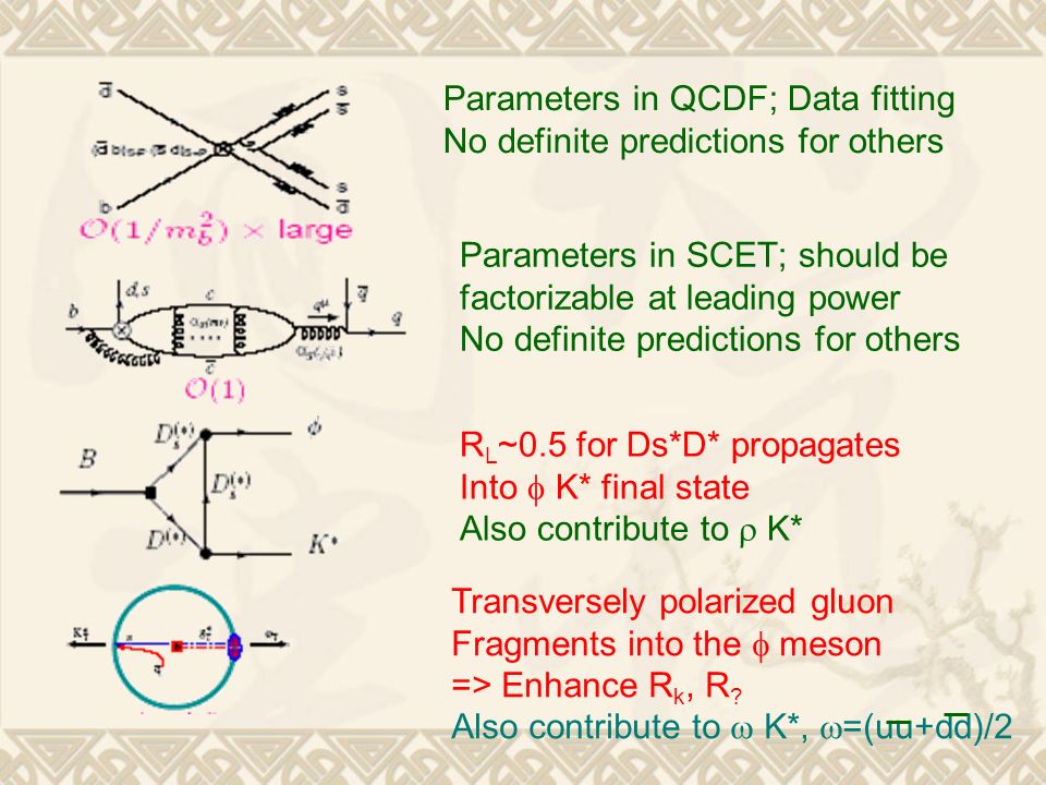
60. Parameters in QCDF; Data fitting No definite predictions for others Parameters in SCET; should be factorizable at leading power No definite predictions for others R L ~0.5 for Ds*D* propagates Into  K* final state Also contribute to  K* Transversely polarized gluon Fragments into the  meson => Enhance R k, R ? Also contribute to  K*,  =(uu+dd)/2

62. Thank You