1. Summary Remote Sensing Seminar Summary Remote Sensing Seminar Lectures in Maratea Paul Menzel NOAA/NESDIS/ORA 22-31 May 2003

2. Observations depend on telescope characteristics (resolving power, diffraction) detector characteristics (signal to noise) communications bandwidth (bit depth) spectral intervals (window, absorption band) time of day (daylight visible) atmospheric state (T, Q, clouds) earth surface (Ts, vegetation cover) Satellite remote sensing of the Earth-atmosphere

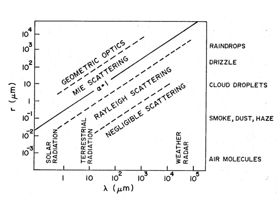
3. Spectral Characteristics of Energy Sources and Sensing Systems

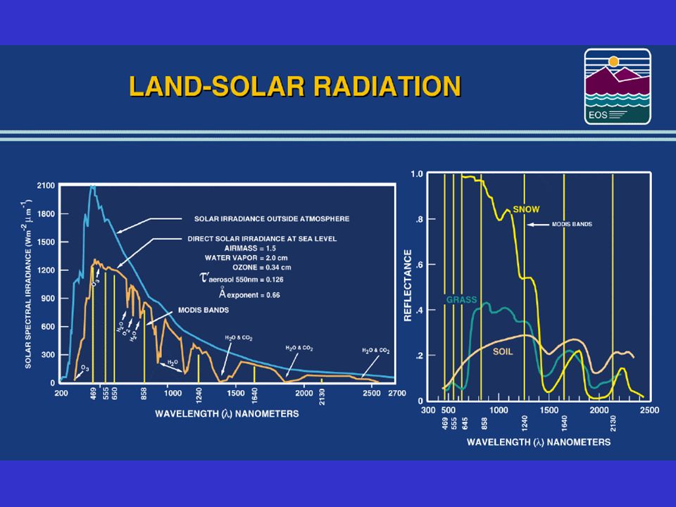
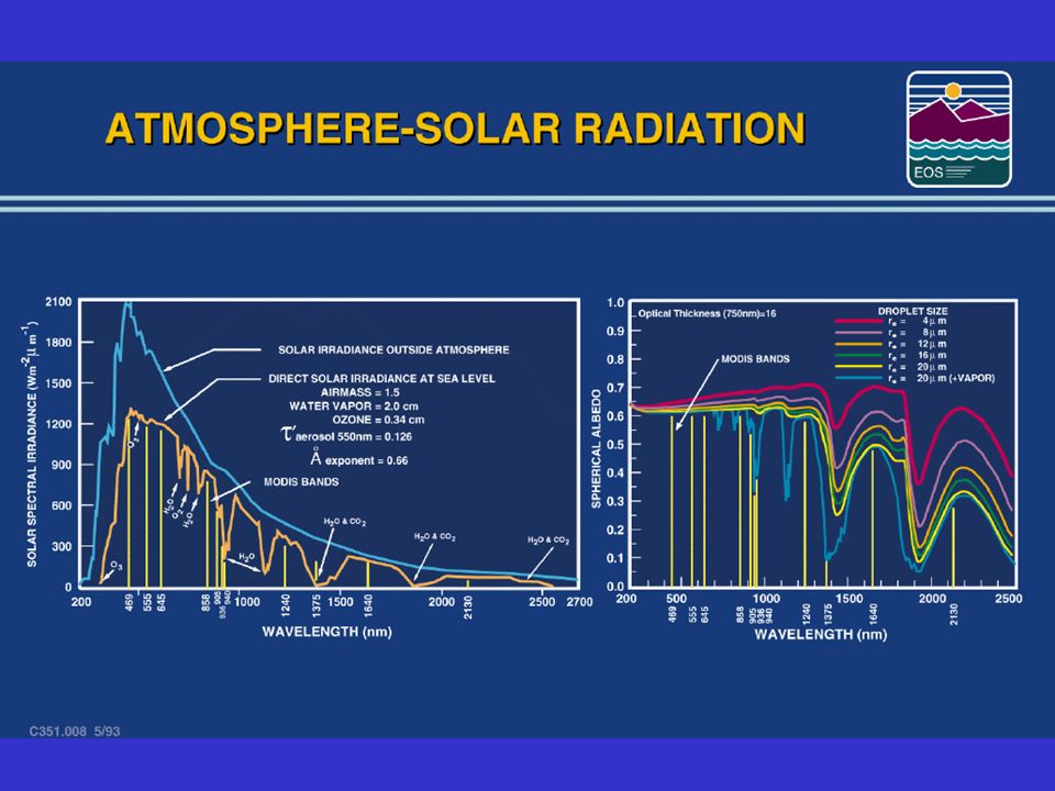
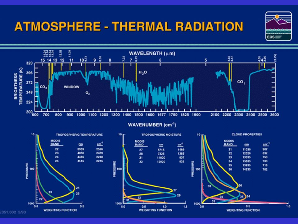
4. Incoming solar radiation (mostly visible) drives the earth-atmosphere (which emits infrared). Over the annual cycle, the incoming solar energy that makes it to the earth surface (about 50 %) is balanced by the outgoing thermal infrared energy emitted through the atmosphere. The atmosphere transmits, absorbs (by H2O, O2, O3, dust) reflects (by clouds), and scatters (by aerosols) incoming visible; the earth surface absorbs and reflects the transmitted visible. Atmospheric H2O, CO2, and O3 selectively transmit or absorb the outgoing infrared radiation. The outgoing microwave is primarily affected by H2O and O2. Solar (visible) and Earth emitted (infrared) energy

5. Solar Spectrum

6. VIIRS, MODIS, FY-1C, AVHRR H2O O2 CO2 H2O O2 H2O O2

7. AVIRIS Movie #2 AVIRIS Image - Porto Nacional, Brazil 20-Aug-1995 224 Spectral Bands: 0.4 - 2.5  m Pixel: 20m x 20m Scene: 10km x 10km

8. MODIS IR Spectral Bands MODIS

9. Current GOES Sounder Spectral Bands: 14.7 to 3.7 um and vis

10. GOES Sounder Spectral Bands: 14.7 to 3.7 um and vis

11. Radiative Transfer through the Atmosphere

12. II II I |I IATMS Spectral Regions

14. Radiation is governed by Planck’s Law c 2 / T B(,T) = c 1 /{ 5 [e -1] } In microwave region c 2 /λT << 1 so that c 2 / T e = 1 + c 2 /λT + second order And classical Rayleigh Jeans radiation equation emerges B λ (T)  [c 1 / c 2 ] [T / λ 4 ] Radiance is linear function of brightness temperature.

20. Multispectral data reveals improved information about ice / water clouds

21. MODIS

23. Ice reflectance

26. Using wavenumbers c 2 /T Planck’s Law B(,T) = c 1 3 / [e -1] (mW/m 2 /ster/cm -1 ) where = # wavelengths in one centimeter (cm-1) T = temperature of emitting surface (deg K) c 1 = 1.191044 x 10-5 (mW/m 2 /ster/cm -4 ) c 2 = 1.438769 (cm deg K) Wien's Law dB( max,T) / dT = 0 where (max) = 1.95T indicates peak of Planck function curve shifts to shorter wavelengths (greater wavenumbers) with temperature increase.  Stefan-Boltzmann Law E =   B(,T) d =  T 4, where  = 5.67 x 10-8 W/m2/deg4. o states that irradiance of a black body (area under Planck curve) is proportional to T 4. Brightness Temperature c 1 3 T = c 2 /[ln( ______ + 1)] is determined by inverting Planck function B

27. Radiative Transfer Equation When reflection from the earth surface is also considered, the RTE for infrared radiation can be written o I =  sfc B (T s )  (p s ) +  B (T(p)) F (p) [d  (p)/ dp ] dp p s where F (p) = { 1 + (1 -  ) [  (p s ) /  (p)] 2 } The first term is the spectral radiance emitted by the surface and attenuated by the atmosphere, often called the boundary term and the second term is the spectral radiance emitted to space by the atmosphere directly or by reflection from the earth surface. The atmospheric contribution is the weighted sum of the Planck radiance contribution from each layer, where the weighting function is [ d  (p) / dp ]. This weighting function is an indication of where in the atmosphere the majority of the radiation for a given spectral band comes from.

28. RTE in Cloudy Conditions I λ = η I cd + (1 - η) I c where cd = cloud, c = clear, η = cloud fraction λ λ o I c = B λ (T s )  λ (p s ) +  B λ (T(p)) d  λ. λ p s p c I cd = (1-ε λ ) B λ (T s )  λ (p s ) + (1-ε λ )  B λ (T(p)) d  λ λ p s o + ε λ B λ (T(p c ))  λ (p c ) +  B λ (T(p)) d  λ p c ε λ is emittance of cloud. First two terms are from below cloud, third term is cloud contribution, and fourth term is from above cloud. After rearranging p c dB λ I λ - I λ c = ηε λ   (p) dp. p s dp Techniques for dealing with clouds fall into three categories: (a) searching for cloudless fields of view, (b) specifying cloud top pressure and sounding down to cloud level as in the cloudless case, and (c) employing adjacent fields of view to determine clear sky signal from partly cloudy observations.

29. Cloud Properties RTE for cloudy conditions indicates dependence of cloud forcing (observed minus clear sky radiance) on cloud amount (  ) and cloud top pressure (p c ) p c (I - I clr ) =    dB. p s Higher colder cloud or greater cloud amount produces greater cloud forcing; dense low cloud can be confused for high thin cloud. Two unknowns require two equations. p c can be inferred from radiance measurements in two spectral bands where cloud emissivity is the same.  is derived from the infrared window, once p c is known. This is the essence of the CO2 slicing technique.

30. Cloud Clearing For a single layer of clouds, radiances in one spectral band vary linearly with those of another as cloud amount varies from one field of view (fov) to another Clear radiances can be inferred by extrapolating to cloud free conditions. R CO2 R IRW cloudy clear x xx x x partly cloudy N=1N=0

31. Moisture Moisture attenuation in atmospheric windows varies linearly with optical depth. - k u  = e = 1 - k u For same atmosphere, deviation of brightness temperature from surface temperature is a linear function of absorbing power. Thus moisture corrected SST can inferred by using split window measurements and extrapolating to zero k Moisture content of atmosphere inferred from slope of linear relation.

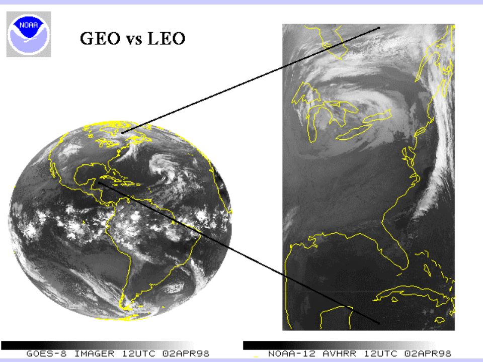
33. Comparison of geostationary (geo) and low earth orbiting (leo) satellite capabilities GeoLeo observes process itselfobserves effects of process (motion and targets of opportunity) repeat coverage in minutesrepeat coverage twice daily (  t  30 minutes)(  t = 12 hours) full earth disk onlyglobal coverage best viewing of tropicsbest viewing of poles same viewing anglevarying viewing angle differing solar illuminationsame solar illuminationvisible, IR imager (1, 4 km resolution)(1, 1 km resolution) one visible bandmultispectral in visible (veggie index) IR only sounder IR and microwave sounder (8 km resolution)(17, 50 km resolution) filter radiometerfilter radiometer, interferometer, and grating spectrometer diffraction more than leo diffraction less than geo

34. 35_98 34 Email comments on course to paoloa@ssec.wisc.edu Best feature Worst feature Suggestions to improve