1. MODIS/AIRS Workshop MODIS Level 2 Cloud Product 6 April 2006 Kathleen Strabala Cooperative Institute for Meteorological Satellite Studies University of Wisconsin-Madison USA

2. Day 3 Lecture Outline Review of MODIS atmosphere products MODIS Level 2 product theory and algorithms –MODIS Cloud Top Properties Product –MODIS Cloud Phase Product –MODIS Aerosol Product Example of MODIS aerosol application –MODIS Atmospheric Profiles Product MODIS Ocean Products –SeaDAS

3. MODIS Standard Products Atmosphere MOD 04 - Aerosol Product MOD 05 - Total Precipitable Water (Water Vapor) MOD 06 - Cloud Product * (CTP & IRPHASE only)MOD 06 - Cloud Product MOD 07 - Atmospheric Profiles MOD 08 - Gridded Atmospheric Product MOD 35 - Cloud Mask

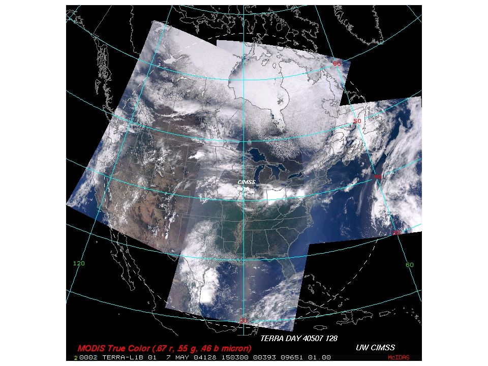
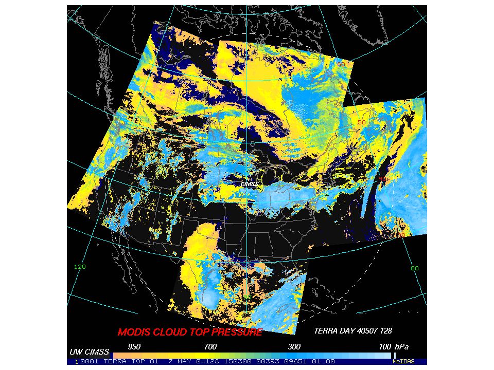
4. Cloud Top Properties Menzel, Wylie - CIMSS Cloud Top Pressure, Temperature, Emissivity derived using CO 2 “slicing” MODIS product utilizes 4 spectral channels in the 13 – 14  m region. 5x5 1 km pixel retrievals where at least 5 of the 1 km pixels are cloudy as determined by the cloud mask Cloud properties retrieved both day and night

5. Inputs MODIS L1B (MOD021KM) and geolocation file (MOD03) MODIS Cloud Mask (MOD35) 6 hourly Global Data Assimilation System T126 resolution analysis from NCEP (Vertical Profiles of Temperature and Moisture) ex : gdas1.PGrbF00.020430.00z Weekly Optimum Interpolation (OI) Sea Surface Temperature (SST) Analysis ex: oisst.20050608 Latest 7 days ancillary data and documentation available from: ftp://aqua.ssec.wisc.edu/pub/terra/ancillary

7. CO2 channels see to different levels in the atmosphere 14.2 um 13.9 um 13.6 um 13.3 um

8. Radiative Transfer Equation The radiance leaving the earth-atmosphere system sensed by a satellite borne radiometer is the sum of radiation emissions from the earth-surface and each atmospheric level that are transmitted to the top of the atmosphere. Considering the earth's surface to be a blackbody emitter (emissivity equal to unity), the upwelling radiance intensity, I, for a cloudless atmosphere is given by the expression I =  sfc B ( T sfc )  (sfc - top) +   layer B ( T layer )  (layer - top) layers where the first term is the surface contribution and the second term is the atmospheric contribution to the radiance to space.

9. When reflection from the earth surface is also considered, the Radiative Transfer Equation for infrared radiation can be written o I =  sfc B (T s )  (p s ) +  B (T(p)) [d  (p)/ dp ] dp p s where F (p) = { 1 + (1 -  ) [  (p s ) /  (p)] 2 } The first term is the spectral radiance emitted by the surface and attenuated by the atmosphere, often called the boundary term and the second term is the spectral radiance emitted to space by the atmosphere directly or by reflection from the earth surface. The atmospheric contribution is the weighted sum of the Planck radiance contribution from each layer, where the weighting function is [ d  (p) / dp ]. This weighting function is an indication of where in the atmosphere the majority of the radiation for a given spectral band comes from.

10. Radiative Transfer Equation I =  sfc B (T s )  (p s ) +  B (T(p)) [d  (p)/ dp ] dp RTE in Cloudy Conditions I λ = η I cd + (1 - η) I clr where cd = cloud, clr = clear, η = cloud fraction λ λ o I clr = B λ (T s )  λ (p s ) +  B λ (T(p)) d  λ. λ p s p c I cd = (1-ε λ ) B λ (T s )  λ (p s ) + (1-ε λ )  B λ (T(p)) d  λ λ p s o + ε λ B λ (T(p c ))  λ (p c ) +  B λ (T(p)) d  λ p c ε λ is emittance of cloud. First two terms are from below cloud, third term is cloud contribution, and fourth term is from above cloud. After rearranging p c dB λ I λ cd - I λ clr = ηε λ   (p) dp. p s dp

11. Cloud Properties from CO2 Slicing RTE for cloudy conditions indicates dependence of cloud forcing (observed minus clear sky radiance) on cloud amount (  ) and cloud top pressure (p c ) p c (I - I clr ) =    dB (T). p s Higher colder cloud or greater cloud amount produces greater cloud forcing; dense low cloud can be confused for high thin cloud. Two unknowns require two equations. p c can be inferred from radiance measurements in two spectral bands where cloud emissivity is the same.  is derived from the infrared window, once p c is known.

12. Different ratios reveal cloud properties at different levels hi - 14.2/13.9 mid - 13.9/13.6 low - 13.6/13.3 Meas Calc p c (I 1 -I 1 clr )  1   1 dB 1 p s ----------- = ---------------- p c (I 2 -I 2 clr )  2   2 dB 2 p s

13. BT in and out of clouds for MODIS CO 2 bands - demonstrate weighting functions and cloud top algorithm S. Platnick, ISSAOS ‘02

14. MODIS Cloud Top Properties Level 3 Products March 2004

17. Cloud Top Temperature Plymouth Marine Lab, UK 10 October 2003 11:57 UTC http://www.npm.ac.uk/rsg/projects/cloudmap2/

18. Output Product Description

19. MOD06 Key Output Parameters 5x5 pixel (1km) resolution Surface_Temperature (GDAS input) Surface_Pressure (GDAS input) Cloud_Top_Pressure Cloud_Top_Temperature Tropopause_Height Cloud_Fraction Cloud_Effective_Emissivity Cloud_Top_Pressure_Infrared Brightness_Temperature_Difference_B29-B31 Brightness_Temperature_Difference_B31-B32 Cloud_Phase_Infrared Cloud Optical Depth (daytime – 1 km product) Cloud Effective Radius (daytime – 1km)

20. Known Problems Low cloud –Vantage point of satellite means more sensitive to high cloud than low cloud. New algorithm address this Solution converges on highest pressure level – Addressed with latest algorithm

21. Validation - Comparison of HIRS/ISCCP/MODIS High Cloud Frequency July 2002December 2002

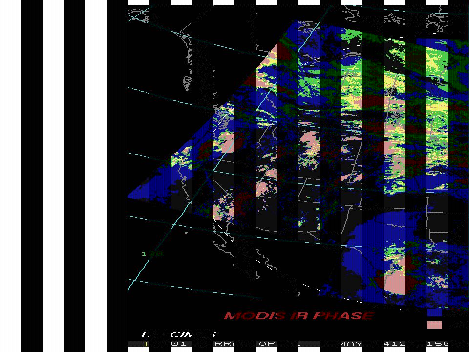
22. Cloud Phase Dr. Bryan Baum CIMSS Based upon the differential absorption of ice and water between 8 and 11 microns Simple brightness temperature difference (8-11 BTDIF) technique Included as part of the MOD06 product

23. Imaginary Index of Refraction of Ice and Water 8 – 13 microns

24. High Ice clouds BTD[8.5-11] > 0 over a large range of optical thicknesses  T cld = 228 K Midlevel clouds BTD[8.5-11] values are similar (i.e., negative) for both water and ice clouds T cld = 253 K Low-level, warm clouds BTD[8.5-11] values always negative T cld = 273 K Ice: Cirrus model derived from FIRE-I in-situ data ( Nasiri et al, 2002) Water: r e =10  m Angles   = 45 o,  = 20 o, and  40 o Profile: midlatitude summer Simulations of Ice and Water Phase Clouds 8.5 - 11  m BT Differences  =

25. Ice Cloud Example

26. Water Cloud Example

27. IRPHASE Thresholds Ice Cloud –BT11 0.5 K Mixed Phase –BT11 between 238 and 268 K and –BTD8-11 between –0.25 and –1.0 K Water Cloud –BT11 > 238 K and BTD8-11 < -1.5 K or –BT11>285 and BTD8-11 < -0.5 K

28. Output Product Description 4 categories 1 – Water Cloud 2 – Ice Cloud 3 – Mixed Phase Cloud 6 – Undecided

29. MOD06 Key Output Parameters 5x5 pixel (1km) resolution Surface_Temperature (GDAS input) Surface_Pressure (GDAS input) Cloud_Top_Pressure Cloud_Top_Temperature Tropopause_Height Cloud_Fraction Cloud_Effective_Emissivity Cloud_Top_Pressure_Infrared Brightness_Temperature_Difference_B29-B31 Brightness_Temperature_Difference_B31-B32 Cloud_Phase_Infrared Cloud Optical Depth (daytime – 1 km product) Cloud Effective Radius (daytime – 1km)

30. Temperature sensitivity, or the percentage change in radiance corresponding to a percentage change in temperature, , is defined as dB/B =  dT/T. The temperature sensivity indicates the power to which the Planck radiance depends on temperature, since B proportional to T  satisfies the equation. For infrared wavelengths,  = c 2 /T = c 2 / T. __________________________________________________________________ Wavenumber Typical Scene Temperature Temperature Sensitivity 700 (14  m)220 4.58 900 (11  m) 300 4.32 1200 (8.3  m) 300 5.76 1600 (6.5  m) 240 9.59 2300 (4.4  m) 22015.04 2500 (4.0  m) 30011.99

31. MODIS IR Spectral Bands MODIS

32. Cloud edges and broken clouds appear different in 11 and 4 um images. T(11)**4=(1-N)*Tclr**4+N*Tcld**4~(1-N)*300**4+N*200**4 T(4)**12=(1-N)*Tclr**12+N*Tcld**12~(1-N)*300**12+N*200**12 Cold part of pixel has more influence for B(11) than B(4) Warm part of pixel has more influence for B(4) than B(11)

33. Ice Cloud Example

34. Broken clouds appear different in 8.6, 11 and 12 um images; assume Tclr=300 and Tcld=230 T(11)-T(12)=[(1-N)*B11(Tclr)+N*B11(Tcld)] -1 - [(1-N)*B12(Tclr)+N*B12(Tcld)] -1 T(8.6)-T(11)=[(1-N)*B8.6(Tclr)+N*B8.6(Tcld)] -1 - [(1-N)*B11(Tclr)+N*B11(Tcld)] -1 Warm part of pixel has more influence at shorter wavelengths 8.6-11 11-12 N=0 N=0.2 N=0.8 N=0.6 N=0.4 N=1.0

35. Known Problems Mid-level cloud (BT ~ 250 K) –Ambiguous solution Surface Emissivity Effects –Not always the same over the IR window (granite) Mixed phase cloud category –should be considered as undecided

37. Cloud Phase Level 3 Product March 2004 Water Ice