1. CM30075: Computer Graphics www.bath.ac.uk/~maspmh/
Peter Hall

2. !! Warning !! These slides do not replace text book reading

3. L01: about this course
Aim: to teach the elements of Computer Graphics Traditional 3D photorealism Modern use of images, and non-photorealism
Method: traditional forms lectures personal reading personal practical work
Assumptions: knowledge of analytic mathematics vectors and matrices integration and differentiation

4. curriculum 1. Traditional Photorealism 1.1 Modelling
1.1.1 B-rep (02,09)
1.1.2 CSG (10)
1.1.3 Voxels (10)
1.1.4 Texture Maps (11)
1.2 Lighting
1.2.1 Simple reflection models (05)
1.2.2 Advanced reflection and refraction, BRDF (07)
1.2.3 The lighting equation (08)
1.3 Rendering
1.3.1 Cameras and Projection (03)
1.3.2 Ray tracing (06)
1.3.3 Hidden surfaces and Cast Shadows (04)
1.3.4 Radiosity (08)
1.4 Animation
1.4.1 Animation Basics (12)
1.4.2 Articulated figures (13)
1.4.3 Soft objects and Fluids (14)
1.4.4 Fire and Smoke (15)
2. Modern Topics
2.1 Interaction with photographs
2.1.1 Compositing (16)
2.1.2 Making panoramas (17)
2.1.3 Intelligent scissors (18)
2.1.4 Texture propagation (19)
2.2 Non-photorealistic Rendering
2.2.1 From 3D models (20)
2.2.2 From images and video (21)
2.2.3 Generalised Cameras (22)
A. Mathematical Appendix
A.1 Useful geometry of points, lines and planes. (04)

5. Traditional Computer Graphics
Lecture number / curriculum index
Topic
Learning objective
01 / 1
Introduction to CM30075
And Compuer Graphics
Pointers to course materials given., Traditional Graphics outlined briefly.
Traditional Computer Graphics
02 / 1.1.1
Modelling – Brep
The B-rep modelling scheme is introduced as just one way to build objects.
03 / 1.3.1
Rendering – cameras and projection
Camera models introduced. Points are projected, so that objects models can be rendered as wire-frames.
04 / A.1
Rendering – ray-casting
Lines intersected with planar polygons, result used as a basis for ray-casting. Now objects can be rendered to look solid.
05 / 1.2.1
Simple reflection models
Point light sources are introduced; Lambertian and Specular reflection so objects can be shaded.
06 / 1.3.2
Rendering – ray tracing
Cast shadows, reflection and refraction amongst many objects. Ray-tracing as a tree.
Milestone: material for advance practical work is now covered
07 / 1.2.2
Advance lighting and reflection
The BRDF is introduced. Physical models of reflection and refraction.
08 / 1.2.3
The Lighting Equation;
Radiosity
The full complexity of lighting is revealed; radiosity and ray-tracing are seen as specific solutions.
09/ 1.1.1
Modelling revisited – advanced B-rep
Use of spline surfaces as B-rep models; how to define them and how to render them
10/ 1.1.2
Modelling revisited – CSG and Voxels
Voxel models and Volume Rendering
11 / 1.1.3
Texture maps.
Texture maps introduced as things to be rendered that relieve the burden of modelling. Aliasing issue is mentioned.
Milestone: static images now (mostly) covered
12 / 1.4.1
Animation basics
The basics of animation are introduced from both technical and artistic points of view.
13 / 1.4.2
Articulated figures
Modelling bodies and hierarchies of transforms; inverse kinematics/dynamics is discussed
14 / 1.4.3
Soft Objects and Fluids
Elastic properties – use of physics – to model cloth, putty and such like, including fluids.
15 / 1.4.5
Fire and Fluids
Use of dynamic textures and particles to model animate objects with no definitive boundary.
Milestone: Traditional Computer Graphics material covered
Modern Computer Graphics: Photograph editing and non-photorealistic rendering
16 / 2.1.1
Compositing
How images layer to make a whole; simple methods for making panoramas from holiday snaps.
17 / 2.1.2
Panoramic Views
How to make panoramas from holiday snaps – and from video too.
18 / 2.1.3
Intelligent scissors
Cutting and pasting objects in pictures; so more on compositing
19 / 2.1.4
Texture Propagation
Filling in holes in images, maybe left by cutting.
20 / 2.2.1
NPR from 3D models
Why is photorealism the aim? People paint! How to paint, not photograph from models.
21 / 2.2.2
NPR from photos
How can photographs be processed to look like a painting? Why is this difficult?
22 / 2.2.3
Generalised Cameras
The eye of Art is often not a real camera!
Milestone: course content fully introduced
23 revision
24 revision

6. Reading Lecture Slides are NOT intended to replace text book reading.
Standard texts
Watt, 3D Computer Graphics, Addison Wesley.
Foley et al, 3D Computer Graphics, Addison Wesley.
Watt and Watt, Advanced Computer Graphics, Addison Wesley.
For the interested.
SIGGRAPH proceedings (published as journal special issue; Transactions on Graphics)
Eurographics proceedings
IEEE Transactions on Visualization and Computer Graphics
Computer Graphics Forum

7. Practical
Aim: You are to write a simple ray-casting / ray-tracing program.
The practical work is broken into three stages
ray-caster with self-shading
cast-shadows
full ray-tracer.
You should spend no more than 15 hours on this component;
including time to prepare the documents needed for your assessment.

8. Assessment
Assessment will cover all material given in lectures, in assigned reading and in practical work.
75% Sat Examination Questions usually comprise 4 parts: a) Basic knowledge (3rd class) b) Moderate knowledge, basic understanding (2.2nd class) c) Good knowledge / moderate understanding (2.2nd class) d) Good understanding – can solve new problems (1st class)
25% practical work Already explained

9. Computer Graphics Basics
Traditional: What colour is this pixel?
focus
window
object
camera
point (pixel)

10. transform models into place
Rendering Pipeline
Make 3D models
transform models into place
illuminate models
project models
clip invisible parts
raterization
display
The rendering pipeline shows
the flow of information uses
and the processes needed
to synthesise an image.
In fact, there are many rendering pipelines.
The order of processes can change depending, for example, on whether rendering time or rendering quality is more important.
These different pipelines differ only in details – the general flow of information from 3D model to 2D image is always the same.

11. What colour is this pixel?
Modern approaches
What colour is this pixel?
point (pixel)
target image
source image

12. L02: B-rep basics
The B-rep modelling scheme is introduced as just one way to build objects.
points
points and lines
points, lines, and polygons

14. B-rep basics Brep = Boundary Representation
Start with a set of M points p = { (x, y, z)i : i = 1…M }
Make a set of N lines from points L = { (i, j)k : k = 1…N }
Make a set of m polygons from lines B = { (k1, k2, …, kn}l : l = 1…m }
A model is three-dimensional (3D),
if the points are 3D (as above).

15. Different information supports different rendering
points only dots (used in Chemistry, also in modern Point based Rendering)
lines Wire-frame rendering, good for quick tests in animation, say
polygons shaded surfaces
points
points and lines
points, lines, and polygons

16. Practical Issues !! ALWAYS INDEX POINTS !! x1 y1 z1 x2 y2 z2 xi yi zi
polygon table
point table
line table x1 y1 z1 x2 y2 z2 xi yi zi xM yM zM 2 i k 1 3 4 6 8 2 7 *
avoids repeated points, so more efficient
avoids numerical error when animating

17. Different tables can be used
point table
triangle table x1 y1 z1 x2 y2 z2 xi yi zi xM yM zM 1 3 4 7
Triangles are the most common polygon, because triangles are always flat.
But triangles are expensive – many of them; so other polygons used for modelling are often decomposed into triangles for rendering.

19. A Minor Complication !! POINT ORDER MATTERS !! clockwise
anti-clockwise
The ordering gives the polygon a “front” and “back”.
eh! which side is which?

20. The normal of a triangular polygon
The normal of a polygon is used in lighting calculations (and in other calculations too).
Suppose a triangle has points, p, q, r, each point in 3D.
The normal direction is
n = (p-q) x (q-r)
where x is the vector cross product.
Exercise: Show that reversing the order of points also reverses the direction of the normal.

21. build a table of triangles from these points1
Exercise: The points are randomly numbered.
From the view given, point 4 is at the back of the cube, point 5 is the nearest corner.
Build a table of triangles in which vertices are consistently ordered clockwise, when each face of the cube is viewed from the outside. 2 6 4 5 7 3 8

22. B-rep basics: summary B-rep = boundary representation
Models objects with points, lines, polygons
Points are ordered around a polygon
Best to index into tables
The form of tables dictates rendering algorithms
Exercise: Build a 3D cube from well ordered triangles, render it as a wire-frame. See L03 for projection methods.

24. L03: Cameras and Projection
Camera models introduced.
Points are projected, so that objects models can be rendered as wire-frames.

25. The Linear Camera In a linear camera
rays of light travel in straight lines from a object
the camera captures all rays passing through a single focus
intersect a planar window to make the image
the normal from the plane to the focus is the optical axis
focus
window
object
image
ray
optical axis

26. The Linear Camera Two variants exist:
the “physical” model – shown in the previous slide has the focus between the object and the window, in which the image is inverted
the “mathematical model” – which we use, is shown below has the window between the object and focus leaving the image the right way up
focus
window
object
image

27. Basic Perspective Projection
Uses similar triangles to compute the height of the image
object
image
focus

28. 3D is almost as easy as 2D
In the canonical camera, focal length (f) is taken as 1.

29. Homogeneous Points Make projection easy and convenient
3D point (x, y, z) written as (x,y,z,1)
homogeneous point (x, y, z, a) maps to real point 1/a (x, y, z)
The homogeneous points p = (x,y,z,1) and q = (sx, sy, sz, s)
differ only by a scale factor s;
this makes them equivalent in homogenous space.
Notice (x,y,z) and (sx,sy,sz) are two points on the same straight line passing through the origin. This makes them equivalent – they represent the same line!
In homogeneous space, lines and points are dual concepts!

30. A little homogeneous geometry
the set of all rays project
normally onto the window
to make a pattern of “spokes”
object point
a scaled version of the image
straight line (a ray of light)
image point
a scaled version of the object
window
focus:
at the origin
a particular line – the optical axis – passes
normally through the window and through the
focus. This line has the image of the focus –
a vanishing point.

31. Projection with a matrix
Using homogeneous coordinates, projection can be written as a matrix
we do need to divide by homogeneous depth, a, after this
Compare this to with f = 1.

32. The camera as a matrix
Using a matrix for projection is very convenient in many ways.
It means we can model the camera as a matrix, C, say. Now projection of a homogenous point p is just q = pC and we know that the homogeneous image point q is just a scale factor away from being correct – and all we need do is scale it by its depth (last element).
It means we can move the camera about in space just by pre-multiplying by a matrix transform q = pMC
It means we can change the internals of the camera (focal length, aspect ratio, etc) by post-multiplying by a matrix q = pMCK
We can do all of this at once! just set A = MCK, now A is a linear camera q = pA

33. Some Examples Setting using
rotates then translates the camera before projection.
Notice this is equivalent to applying M-1 to the point.

34. Another example
To change focal length, set
now post-multiply

35. All at once
Define a new linear projective camera in a new place and with a new focal length
It is easy to use this camera…
Of course, you can set M and K as you please
– not just rotate and translate and new focal length!
Exercise: See notes for an exercise

36. Rendering with a Projection Matrix
If we had a model built just of points (no lines, planes etc) then we could make a simple images using this simple technique:
Project all points using the projection matrix
Keep all points that lie within the window bounds
Connect points in the picture that are connected in 3D
This produces a “wire frame” picture – easy, and fast!
If all pixels inside a projected triangle can be identified, then they too can be coloured.
This is the basis of scan-conversion.

37. L04: Ray-Casting Lines are intersected with planar polygons.
The result used as a basis for ray-casting.
Now objects can be rendered to look solid.

38. Ray-casting algorithm
For each pixel Cast a ray from the focus through the pixel Compute all intersections with all polygons Find the nearest polygon Colour pixel with polygon colour
Actually, the polygon colour is modified to create the effect of shading, as on a sphere.

39. Ray Casting Basics One ray per pixel, cast into the scene
Look for nearest intersection
Colour pixel accordingly
scene of objects
camera
pixel
focus
window
Expensive part: computing the intersection of a ray with a polygon

40. Line / Polygon intersection
an infinitely wide plane
an infinitely long line
x(s) p r
compute scale factor
Given the scale factor,
the intersection is easy to get

41. Point Inside Triangle? outside inside p2 p1 x p3
some “turns” are anti-clockwise,
others are clockwise
all three “turns” are anti-clockwise
direction of turn:
parallel direction of turn, sij > 0:

42. A practical problem i The frame buffer is in the computer.
We imagine casting rays thru’ pixel centres i j
The window is in “space”;
where are pixel centres in space?

43. Solution: recall the camera as a matrix, C = MPK y = xC = ((xM)P)K
external parameters M locates the camera in space M is a 4x4 matrix, (eg rotation) notice M maps a model point in space use the inverse of M to move camera!
a projection P maps 3D points, to the window P is rank degenerate can be (4x3) but usually is (4x4)
internal parameters, maps window points to frame-buffer transform confined to the plane a matrix K (a 3x3 will do!)

44. The internal parameters transform the pixels centres from “frame buffer” coordinates to “window coordinates”.
There is no single “answer” – here I’ve mapped a rectangular frame buffer to a window which is square, so pixels get stretched into rectangles – but you may keep pixels square.
It is very common (almost universal) to “flip” coordinates so pixel (j,i) maps to location (x,y);
and notices row (j) increase going DOWN - take care when designing K! y i K j x
K-1
point is at (x,y)
pixel is typically at (j,i)

45. The external parameters transforms the canonical camera
in “camera space” to the desired camera in “world space”. M
M-1

46. Ray-casting takes a long time
Why does ray-casting take so long?
Because every ray is compared to every polygon.
Is this necessary?
What are bounding spheres?
Homework question: what is a BSP tree?

47. L05: Simple Reflection Point light sources are introduced.
Lambertian and Specular reflection, so objects can be shaded.

48. Point light sources
A point light source is, er, a point (x,y,z) that emits light.
Actually the point light can be at infinity (think of the sun), in which case (x,y,z) is its direction.
Most point lights sources are often at infinity in computer graphics. This makes shading/reflection efficient to compute because the direction of the light is the same for every intersection point.

49. Basic Reflection Model
light direction
surface normal
mirror direction
Mirror reflection - specular reflection – Phong reflection
Diffuse refection – Lambertian reflection

50. Diffuse/Lambertian Reflection
A beam of light spreads over an area, and is reflected equally in all directions.
So here we’ve not drawn any reflected direction
over a narrow area
over a wide area
these beams
are of equal width
The energy in the light is spread out more over the wider area.
So, the area will appear less bright.

51. Functional analogy: the sun warms the earth more near the equator than the pole
h = w/cos(q) w
The light energy in the beam of width w is spread over a length h = w/cos(q).
Energy density in beam: I/w
Energy density on ground: I/h = Icos(q)/w

52. Lambertian reflection in Graphics
We know that light from the source strikes a surface, to be spread equally
in all directions. So, only the angle between the light direction and the
surface is important.
Iout = Ilightcos(q)
The cosine we need is the dot (inner) product of the unit normal and
unit vector pointing to the light.
Iout = Ilight n.l
BUT the surface can absorb some light, so only a fraction c is reflected
Iout = cIlight n.l
The “diffuse reflection coefficient” c depends on the surface material.

53. Diffuse reflection in colour
To handle colour is easy: just do the same calculation for each colour channel
Rout = credRlight n.l
Gout = cgreenGlight n.l
Bout = cblueBlight n.l
For white light, Rlight = Glight = Blight.
The coefficients c are often thought of as the colour of the material.

54. Specular Reflection
How much light is reflected in a particular direction?
mirror direction, r
light direction, l
surface normal, n
eye direction, e
Intuitively, the angle between the mirror and eye directions is important.
Homework: The eye direction is a given, what is the mirror direction?

55. Phong Reflection Iout = kIlight(r.e)n
Phong’s specular reflection model
Iout = kIlight(r.e)n
Notice how the cosine (r.e) is used.
k is the “specular reflection coeffiecient” for the surface.
Phong reflection works for colour
in just the same sort of way as Lambertian reflection

56. A complete but simple reflection model
A complete model (for a single colour channel) is
Iout = aIamb+ cIlight n.l + kIlight(r.e)n
We see the diffuse and specular terms are added up.
There is an additional term for “ambient” light
this is light that comes equally from every direction
ambient light allows us see the very darkest regions of a picture
Specular highlights often look white, (just look around at things to see this) so k is often given the same value in every colour channel

57. L06: Ray-tracing Ray-tracing is a global lighting method. Cast shadows
Reflection and refraction amongst many objects.
Ray-tracing as a tree.

58. Cast Shadows
Is the box resting on the table ?

59. Is a point in shadow? point light point light
A point is in shadow if the line between it and a light is blocked by an object

60. How can we tell? The point to light ray is a line
Look for intersections of the this line with any object
This is almost an exact repetition of the ray-casting,
except intersections need not be ordered,
just finding one is enough

61. Reversibility of light
Ray tracing relies on a physical principle:
a ray of light can be traced in either direction
So, if a ray of light splits into two parts then its energy is divided.
But we can “run this backwards” and add up the energy in the divided rays to get the energy in the original.
The paths of the light rays are identical, backwards or forwards.

62. Ray tracing extends ray casting
eye
window
object
ray
intersection
refracted ray
reflected ray

63. Ray tracing tree
A ray/object intersection generate a new (reflected, refracted) pair of rays.
These new rays also intersect to generate new rays, hence a tree
Stop when a ray “leaves” the scene, or a set depth
the root
original ray from eye thru’ pixel
intersection
reflected
refracted
intersection
reflected
refracted
intersection
a “parent” ray
when going
UP the tree
reflected
refracted
intersection
a leaf

64. Using the tree in a simple way
The ray-tracing tree is used “bottom up”, from the leaves to the root.
There are no reflected or refracted rays at a leaf.
You can work out the light to the parent using the simple lighting model.
But now the direction to the eye is in fact the direction of the parent ray.
The leaf contributes some energy to its parent,
this parent receives light contributions from both its children.
Now work out the simple light model for the parent, as if it was a leaf,
Add this to the contributions from its children.
And so on.

65. A detail of the tree non-leaf intersection local light + child rays
to parent
surface
leaf intersection
local light only
leaf intersection
local light only
to light
normal
to parent
normal
to parent
mirror
direction
to light
mirror
direction
surface
surface

66. Whitted ray-tracing
Turner Whitted produced the first ray-racer (1980).
It was the first global illumination model. It includes
Hidden surface removal
Self shading (as in diffuse/specular reflection)
Cast shadows
Reflection and refraction (making the model “global”)
The full coursework is to write a Whitted ray-tracer.
A restriction is to not include reflection and refraction, which is “advanced” ray casting.
A further restriction include self-shading only, which is “simple” ray-casting, and the minimum required to make a picture of some kind.

67. L07: Advanced Reflection and Refraction
The BRDF is introduced.
Physical models of reflection and refraction are considered.

68. Overall energy transfer
incident light Ein
reflected light, Erefl
refracted light, Erefr
schematically
conservation of energy
Ein = Erefl + Erefr + Eabs

69. Recall the simple lighting model
c = kaIa + Ikd(n.l) + Iks(r.e)a n e
This takes into account
ambient light
diffuse reflection
specular reflection l r
The energy in the colour depends on where the viewer is, e, compared to the reflection r – and hence the light direction l.

70. A visualisation
Suppose we set Ia = 0, I = 1, kd = 1, ks=1, and n.l = 1 Furher, fix r. Now the lighting depends only on e and a. In fact
c = 1 + e.ra
to get a picture of how the energy depends on point of view

71. A more general idea The light energy depends on
the direction of the incident light
the direction of view

72. Diffuse/Specular lighting
diffuse to diffuse
diffuse to specular
specular to specular
specular to diffuse

73. The BDRF BDRF = bi-directional reflectance function f(f1,f2, q1,q2)
f the fraction of light energy transferred from an incident light ray at (f1,f2) to viewing direction (q1, q2)
In the simple model this is (e.r)a in which r depends on input direction l. (Recall computing r from l is a homework!)
A full BDRF is even more complicated – wavelength, polarization…!

74. The importance of the BDRF
The BDRF controls the kind of material an object appears to be made from, for example
plastic
metal
ceramic
The simple model tends to make things look plastic.

75. Where do we get a BRDF from?
BRDF can be measured from the real thing; not easy!
In graphics, “micro-surfaces” can be used to estimate BRDF.
flat surface
…under a microscope
a perfect mirror
each micro-facet a perfect mirror but overall surface is not!
Look up Torrance Sparrow model.
see, eg

76. L08: The rendering equation
The full complexity of global lighting
radiosity in brief
radiosity and ray-tracing as specific solutions
See: Watt & Watt, Advanced Animation and Rendering, subsec 12.2

77. what colour is the light coming out?
Global Lighting
Every object reflects light
(otherwise, it would look like a black hole)
So, every object can be reflected in every other !
This makes global lighting very complicated.
light in
light out
what colour is the light coming out?

78. Scattering, Shadows and refraction complicate further still !
light out
light in
and real cases are still more complicated !

79. Kajya’s rendering equation
The light transported from point y to point x
g(x,y) is the “visibility” function, 0 if x is in shadow wrt y, 1/|y-x|2 otherwise.
e(x,y) is the transfer directly from y to x
r(x,y,z) is BDRF (scattered light) toward x by y given light source at z
S is the set of all points in the scene
Important: I(.,.) appears both sides.

80. Use of Rendering Equation
Different lighting models are special-case solutions:
The local-model
Ray-tracing
Radiosity

81. Solving the rendering equation
rewrite as
with R an integral operator
Now
hence

82. consider
first term – direct (local) lighting: x is the eye, y a point
subsequent terms account for scattering from other points

83. Ray-tracing Forward ray-tracing (from the eye to lights)
specular to specular : bounces, Phong term
specular to diffuse: Lambertian
diffuse to diffuse (but badly!): Ambient
Backward ray-tracing (to the eye from lights)
diffuse to specular

84. light radiates to all other patches
Radiosity
Diffuse to Diffuse
This is the (badly modelled) “ambient” term in “local” models
light falls onto a patch from all others
light radiates to all other patches

85. The light energy per unit area is called radiosity
total energy at a patch is its radiosity x its area
and energy is conserved, so at a patch
radiosity x area = emitted energy + reflected energy

86. In a closed environment the energy transfer between patches will reach an equilibrium.
If we use a discrete environment (ie a finite model), then we can use a discrete form of the radiosity equation
The form factors are correlated:
so that, on division by Ai we get the basic equation used:

87. the radiosity equation in matrix form
the hard part is computing the form factors.
(See a standard text for how to do this)
Once they are at hand, solve the system for the B.
then render with a scan converter.

88. L09: Brep with curves Spline surfaces as B-rep models
How to define them
How to render them

89. Many real world objects are curved.
But so far, we have used flat modelling primitives.
Here, we learn how to use curved primitives.
We first look at curve lines in space,
and then at curved surfaces in space.

90. Both curves and surfaces are collections of points in space.
The points are related to one another by some function or other.
In principle the curves and surfaces contain an infinite number of points, but in practice we are forced to use finitely many points.
And we can think of surfaces as a collection of curves

91. There are many ways to define curves and surfaces
Implicit: “balances” a points coordinates
Unit Circle… x2 + y2 = 1
Unit sphere: x2 + y2 + z2 = 1
We will use implicit forms in CSG modelling.
Here we will use parametric forms.
Parametric forms allow you to compute points directly.
This is much better for Brep models.

92. Parametric forms allow you to compute points directly.
This is much better for Brep models.
Parametric curves require one parameter, u.
x(u)
is a point in 3D, on the curve.
Parametric surfaces require two parameters x(u,v)
is a point in 3D, on the surface.

93. Formally
x(u) is a mapping from the real line, R, to a subset of R3. It’s as if the real line (x axis) is bent into the shape of the curve. u
x(u)
x(u,v) is a mapping from the real plane, R2, to a subset of R3. It’s as if the real plane (xy-plane) is bent into the shape of the curve. u
x(u,v) v

94. This is an abuse of notation!
Curves:
An easy way to specify a curve is with a polynomial; most modellers use cubics:
x(u) = a + bu + cu2 + du3
= [u3 u2 u 1][d c b a]
The coefficients a, b, c, d specify the curve.
But this is not the most convenient way, because it’s hard to control. So the cubic is usually specified in some other way.
This is an abuse of notation!

95. Bezier Curves and Surfaces are just one of the many alternatives
x(u) = UMP
U = [u3 u2 u 1]
M = [ ]
P = [p p p p3]
parameter vector
the “Bezier” matrix
4 control points

96. Examples of Bezier curves
control points
Bezier curve

97. Bezier surfaces
analogous issues over control of surfaces argue in favour of,
say, Bezier surfaces; again one of may controllable forms.
x(u,v) = UMPMtVt
The M is the Bezier matrix,
U and V parameter vectors,
P is now a 4x4 matrix of control points.

98. A Bezier surface example

99. Rendering curved surfaces
Can compute intersection of ray/patch but this is difficult and expensive.
More often, the surface is broken into many small triangles; the approximation error is carefully controlled.
Homework: read and summarise (for yourself) one method for decomposing a surface into triangles.

100. Computing normals of surfaces
Could use normal from a triangle. Better to get the normal at a point directly.
compute partials (only one is shown)
get normal direction

101. Issues not considered here:
Stitching patches together to make a bigger surface. Continuity issues constrain the points around the joins.
The differential geometry of curves and surfaces Frenet frames Gaussian curvature

102. L10: CSG and Voxels
Construct Solid Geometry basics
Voxel models

103. CSG basics
Brep is not the only way to represent objects. CSG is another common way.
CSG is models define sets of points via inequalities.
Example
A straight line, y = mx+c, divides the plane:
set f(x,y) = mx + c – y
then f(x,y) > 0 are points above the line f(x,y) = 0 are points on the line f(x,y) < 0 are point below the line

104. More generally
if f(x,y,z) is any scalar function of 3 spatial variables then it can be used to partition space points, using the sign of f(x,y,z).
More examples:
unit sphere: f(x,y,z) = x^2 + y^2 + z^2 – 1
unit cylinder: f(x,y,z) = x^2 + y^2 – 1

105. Creating new shapes
Let’s write f(x) in place of f(x,y,z); x has become a vector, x = (x,y,z,1).
Now suppose f(x) = x12 + x22 -1, a sphere
And suppose M is a transform,
then f(xM) is a mapped version of the sphere;
is an ellipse – maybe with a new centre.

106. Combining shapes CSG primitives are just sets of points.
So they are easy to combine into more complex shapes.
sphere(.)
cylinder(.)
DIF
doughnut(.)
plane(.)
tetrahedron(.)
AND
Any set operation can be used to combine primitives Any new shapes can be combined too.

107. Ray tracing could be suitable –
Rendering CSG
Ray tracing could be suitable –
the “CSG” plane is already used by us! and bounding spheres are CSG models!
We just have to be clever about following the model tree when deciding if a ray strikes an object (eg dougnut example).
And (partial) differentiating gives normals;
Homework: show the normal at a point x on the unit sphere is 2x.

108. NB: This list is my personal view based on vast non-experience.
CSG vs Brep
CSG
B-rep
points implicit
point explicit
sets easy to handle
sets hard to handle
goodish to ray trace
hardish to ray-trace
hard for radiosity
good for radiosity
easy to combine
hard to combine
hard to get from life
easier to get from life
NB: This list is my personal view based on vast non-experience.

109. Voxel Models A pixel is a picture element – an area of colour
A voxel is a volume element – a volume of colour
Voxels are often (partially) transparent.
Voxels (typcally) come from medical data: CAT - bones MRI – soft tissue

110. a single voxel
many voxels
voxels are arranged into a brick;
each brick can contain hundreds – thousands – of voxels
in each direction

111. Typical rendering: CAT scans
CAT scan data produces voxels with a “density”,
so is a scalar field f(x,y,z).
Use the scalar field to assign colour and opacity
Compute a normal at each voxel Use finite differences for this
Shoot a ray through a pixel into the volume, compute lighting at each voxel integrate colour and opacity over the ray f
colour

112. Example – taken from Wikipedia

113. L11: Texture maps
Texture maps
Variations
Two problems

114. Texture maps: what and why
A texture map is a picture:
a carpet a label on a can of food the earth …many other examples
Texture maps are used where the level detail needed make standard modelling inefficient / impossible.

115. The idea is to “wrap” or “warp” a flat picture onto a 3D surface+
In this example, a texture of the earth is mapped onto a sphere =

116. Variations on a theme Bump mapping Environment mapping
Procedural mapping

117. Two problems
1. Flat pictures will not map onto many (most) surfaces: toroids bunnies etc
2. Aliasing – the texture map is made of pixels the pixels can show up and the texture is squashed / stretched to fit the surface making the problem worse

118. (sort of) solving problem 1
Use “intermediate” shapes, typically sphere cylinder cube y
x is a point on the object
c is the object centre
y is the project of x on the im-shape x c

119. Basic algorithm has two steps:
Map the 2D texture (u,v) to the 3D surface (x,y,z): x = x(u,v), y = y(u,v), z = z(u,v) T(u,v) -> T(x,y,z) This is called the S-mapping
Map the object to the same 3D surface x = x’(xo,yo,zo) y = y’(xo,yo,zo) z = z’(xo,yo,zo) T(x,y,z) -> T(xo,yo,zo) This is called the O-mapping

120. Other O-mappings from the object to im-surface exist
centroid
object normal x
surface normal x x
reflected ray
this one makes reflect the environment

121.
3D textures (procedural)
environment
simple
bump
opacity

122. (sort of) solving problem 2
Recall: Aliasing of textures
solution : mip-mapping
mip = multim im parvo "many things in a small space“
The texture is scaled
and filtered
BEFORE use

123. 1. The texture is scaled
and filtered
2. In use, the program selected the
correct section of the mipmap, according
to distance

124. L12: Animation Basics Animation as an art Animation of solid bodies
Camera motion

125. Animation as an art technically, animation is motion
artistically it means “bring to life”

126. Traditional animators use many tricks to bring their characters to life – to animate them.
All tricks break Physics
ghosting
streak-lines
squash-and-stretch
rubber inertia

128. Animation of solid bodies
This is easy – the same transform is applied to all points
The transform is usually a matrix, but does not have to be.
The transform can be differential
x(t+dt) = f[ x(t) ]
but this often leads to numerical error;
so the transform is more often absolute
x(t) = f[ x(0) ]
The set of point {x(0)} is – conveniently – the “canonical” object

129. Examples
TiRi
RiTi

130. Camera motion Cameras often follow a path through a scene.
The path is often defined by a cubic curve.
But this just says where the camera is, we need to know:
* where it points
* and control the camera speed.
We must return to the differential geometry of a curve...

131. To control speed and acceleration along the curve we need
Arc-Length Parameterisation
Recall the Brep curves; x(u) = U*P is a point on the curve
u is a “natural parameter”
parameterisation is arbitrary
define c(u) as the length of the arc

133. To control viewing direction along the curve
we need
Frenet Frames

134. L13: Articulated Figures
Model Specifications
Hierarchies of transforms
Inverse kinematics/dynamics

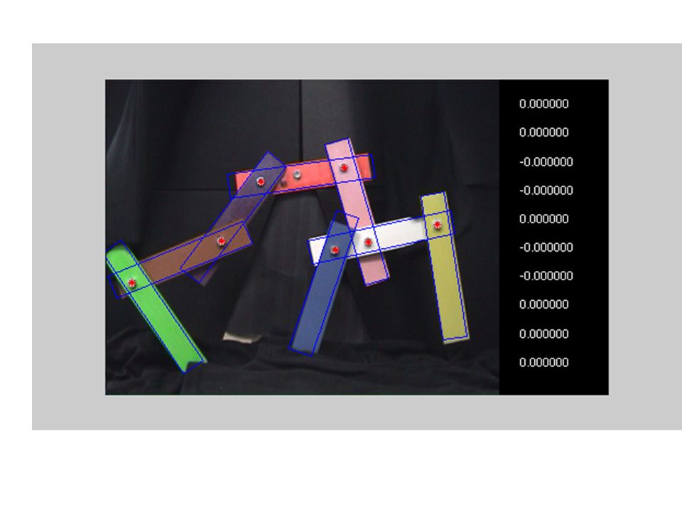
136. Model specifications Articulated models comprise a set of “limbs”
joints that link the limbs
methods to move the limbs
plus appearance information (colour etc)

137. Here the limbs are just rectangles;
limbs that are rigid bodies are much easier to handle
in which case rectangles are OK to use .
So we can think about the joints.
These are specified in many different ways.
Here a joint is just a point
the limbs move around the point
Often within a constrained angle
(In 3D, within a constrained solid angle)

138. The way angles are measured
must be carefully specified.
A frame is needed.
Here the “x” axis runs between joints.
X-axis rotation is, then , angle moved.
parent frame
rotation angle

139. Hierarchies of Transforms
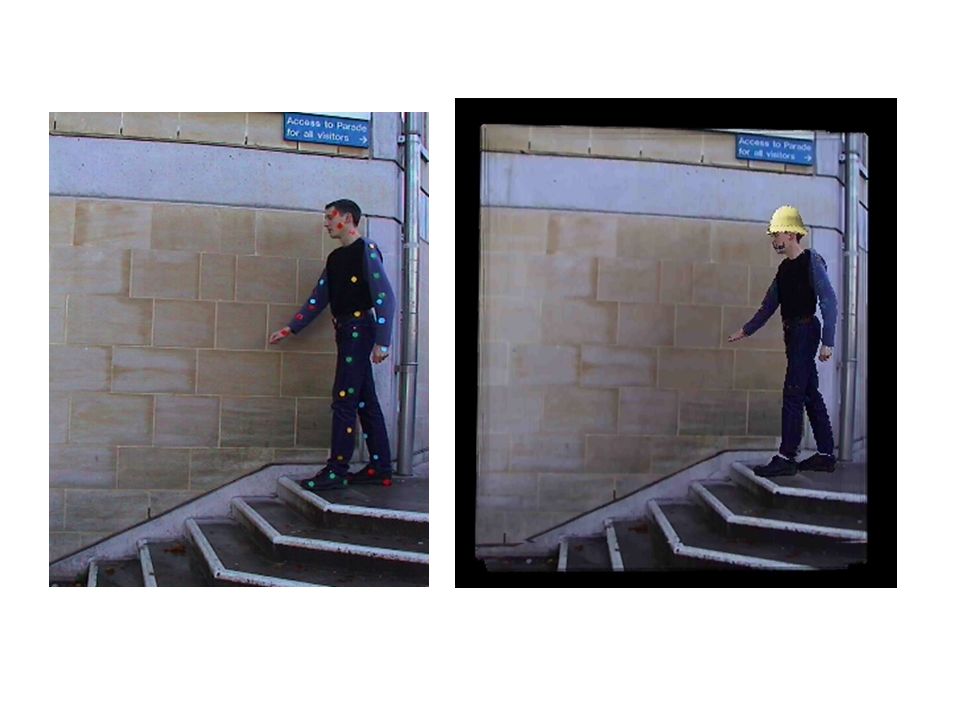
Simple articulated models have a tree-like structure
head
right upper arm
right lower arm
left lower arm
left upper arm
left upper leg
left lower leg
left foot
right upper leg
right lower leg
right foot
body
neck
This tree is used to locate the whole body first, then the next layer of limbs,
and so on. In this tree the feet are placed last of all.

140. Placing a transform at each node in the tree
is a very common method
to make the object move.
We already know how to orient the limb inside its frame,
so all we do is move the frame!
Which way around is correct?
y = xMbodyMupperMlowerMfoot or
y = xMfootMlowerMupperMbody
or will either do? does it matter?

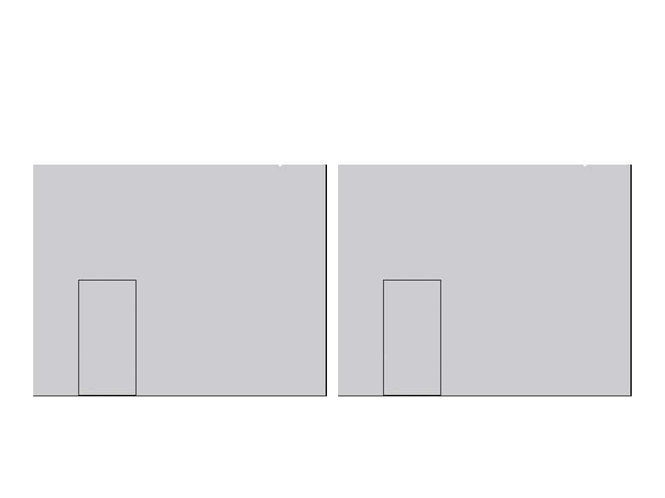
143. Problem:
in the modified video,
why does the foot not goes though the floor?

144. Inverse kinematics/dynamics
Kinematics – the location of the limbs at any given time.
Dynamics – the motion of the limbs at any given time.

145. IK method Put the “puppet” into a poses at various times.
The computer works out how to move from one pose to the next,
in the time available.
The solution has to be subject to some constraints,
typically minimisation of some energy measure.
The method is hard, and tedious – too much so for these note.
See Watt & Watt, section 16.4 for details.

146. L14: Soft Objects and Fluids
Non-physical models
Physical models; elasticity etc for cloth, putty
Water and fluids

147. Soft Objects and Physics
Animation of rigid bodies is easy to achieve;
Animation of articulated figures benefits from “inverse kinematics” and “inverse dynamics”.
Animation of soft objects all but requires the use of physics.

148. Non-physics approaches
Parametric transforms
Spline surfaces
Free-form deformations
Parametric transforms, eg angle of turn about z depend s on z:
R( theta(z) )
Or could animate splines; eg.
Bezier surfaces are easy to move – just move the control points !

149. Free form deformations
FFD’s “move the space”.
FFD’s are tricubic Bezier patches:
Q(u,v,w) = sum sum sum p(i,j,k) Bi(u) Bj(v) Bk(w)
Any point on any object and (u,v,w) maps to the point Q.

150. Physics models Simple use of physics; i) Use Newton’s second law
F = m d2x/dt2
write as a set of first order ODES
F = m du/dt u = dx/dt
ii) Integrate the differential equations over time; setting boundary conditions at time = 0;

151. Elasticity is a well used model
Soft objects are stretchy !!
Force = -k * stretch
Thus given a form for F, motion is determined.

152. Different variants can be – and are - used
Bending forces (twisting forces)

153. Water and fluids The “atom and force” model is good for “soft solids”
But liquids as best modelled in other ways
Again, though, physics is the basis of all the models

154. L15: Fire and Smoke
Not given in 2008

155. L16: NonPhotorealistic Rendering
Why is photorealism the aim? People paint!
What is NPR?
NPR issues

156. Why photorealism? people paint!
Physics provides starting point for models
Photographs provide a foil to test against
But people paint !
Artwork shows off important regions better
Photography is just one depictive style amongst many

157. Which is the simplest to understand?

158. What is NPR?
NPR is a sub-branch of Computer Graphics that studies making images that do not look photographic.
NPR is said to have started around 1990.
Several sub-divisions exist
paint-boxes
rendering 3D models
rendering from photographs and/or video

159. Paint boxes
from the simple…
…to the complex

160. Rendering 3D models
Breslav et al, SIGGRAPH 2007

161. Rendering from photographs and/or video

162. NPR issues NPR depends on perception and interpretation
“drawing implies seeing”
models are much more complex
interaction is common
Mark making
What kind of mark?
Where to mark?
No single foil to test against
there is no “correct” drawing

163. NPR depends on Perception and Interpretation

164. No single foil to test against

165. Mark making: what and where?
What: Emulate real media
pencil, oil paint, chalk, …..
physical models possible
can test for quality of a given mark
What: Produce new media
Can the computer be used to make marks not made before?
Where: Should marks be made locally, globally, or both?
How to decide where to place marks?
Where: How can marks be made stable in animations?

166. L17: NPR from models
The problems
Some solutions

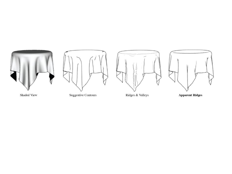
167. The problems Consider a pencil drawing, marks are used to depict:
object boundaries and other contours
shadows and shading
texture

168. Apparent ridges
Judd et al, SIGGRAPH 2007

169. For apparent ridges we need:
differential geometry of surfaces
projection
The curvature at a surface point S(x,y) – how curved is the surface?
Use the Hessian, H, which is a 2x2 matrix of 2nd order partials of S.
The EVD of H = UKUT
principle directions, U = [u1 u2], principle curvature, K = [k1 k2]
Ridges and valleys where k1 is an extremum in direction u1.
Project the local surface geometry (tangents, normals ‘n all),
Look for extremum in this observed geometry.

171. Shadows and shading Shading lines – cross hatches etc
Can be based in “image space”………or in “object space”
Again, curvature can be used, this time to direct pencil lines.

172. Other methods use solid texture maps, that adapt to local lighting and geometry

173. Marks make textures too…
With NPR, even the marks can be animated (look at the sea)

174. L18: NPR from images

175. L18: Smart cut-and-paste

176. L19: Texture Propagation

177. L21: NPR from images

178. L22: Generalised Cameras