1. What we Measure vs. What we Want to Know
"Not everything that counts can be counted, and not everything that can be counted counts." - Albert Einstein

2. Scales, Transformations, Vectors and Multi-Dimensional Hyperspace
All measurement is a proxy for what is really of interest - The Relationship between them
The scale of measurement and the scale of analysis and reporting are not always the same - Transformations
We often make measurements that are highly correlated - Multi-component Vectors

3. Multivariate Description

4. Gulls Variables

5. Scree Plot

6. Output Importance of components:
> summary(gulls.pca2)
Importance of components:
Comp Comp Comp Standard deviation Proportion of Variance Cumulative Proportion
> gulls.pca2$loadings
Loadings:
Comp.1 Comp.2 Comp.3 Comp.4 Weight Wing Bill H.and.B

7. Bi-Plot

8. Environmental Gradients

9. Inferring Gradients from Attribute Data (e.g. species)

10. Indirect Gradient Analysis
Environmental gradients are inferred from species data alone
Three methods:
Principal Component Analysis - linear model
Correspondence Analysis - unimodal model
Detrended CA - modified unimodal model

11. Terschelling Dune Data

12. PCA gradient - site plot

13. PCA gradient - site/species biplot
standard
biodynamic & hobby
nature

14. Making Effective Use of Environmental Variables

15. Approaches
Use single responses in linear models of environmental variables
Use axes of a multivariate dimension reduction technique as responses in linear models of environmental variables
Constrain the multivariate dimension reduction into the factor space defined by the environmental variables

16. Dimension Reduction (Ordination) ‘Constrained’ by the Environmental Variables

17. Constrained?

18. Working with the Variability that we Can Explain
Start with all the variability in the response variables.
Replace the original observations with their fitted values from a model employing the environmental variables as explanatory variables (discarding the residual variability).
Carry our gradient analysis on the fitted values.

19. Unconstrained/Constrained
Unconstrained ordination axes correspond to the directions of the greatest variability within the data set.
Constrained ordination axes correspond to the directions of the greatest variability of the data set that can be explained by the environmental variables.

20. Direct Gradient Analysis
Environmental gradients are constructed from the relationship between species environmental variables
Three methods:
Redundancy Analysis - linear model
Canonical (or Constrained) Correspondence Analysis - unimodal model
Detrended CCA - modified unimodal model

21. Dune Data Unconstrained

22. Dune Data Constrained

23. How Similar are Objects/Samples/Individuals/Sites?

24. Similarity approaches or what do we mean by similar?

25. Different types of data
example
Continuous data : height
Categorical data
ordered (nominal) : growth rate
very slow, slow, medium, fast, very fast
not ordered : fruit colour
yellow, green, purple, red, orange
Binary data : fruit / no fruit

26. Different scales of measurement
example
Large Range : soil ion concentrations
Restricted Range : air pressure
Constrained : proportions
Large numbers : altitude
Small numbers : attribute counts
Do we standardise measurement scales to make them equivalent? If so what do we lose?

27. Similarity matrix
We define a similarity between units – like the correlation between continuous variables.
(also can be a dissimilarity or distance matrix)
A similarity can be constructed as an average of the similarities between the units on each variable.
(can use weighted average)
This provides a way of combining different types of variables.

28. Distance metrics relevant for continuous variables:
Euclidean
city block or Manhattan A B A B
(also many other variations)

29. Similarity coefficients for binary data
simple matching
count if both units 0 or both units 1
Jaccard
count only if both units 1
(also many other variants, eg Bray-Curtis)
simple matching can be extended to categorical data
0,1
1,1
0,0
1,0
0,1
1,1
0,0
1,0

30. A Distance Matrix

31. Uses of Distances Distance/Dissimilarity can be used to:-
Explore dimensionality in data using Principal coordinate analysis (PCO or PCoA)
As a basis for clustering/classification

32. UK Wet Deposition Network

33. Shown with Environmental Variables

34. A Map based on Measured Variables

35. Fitting Environmental Variables

36. Grouping methods

37. Discriminating
If you have continuous measurements and you know which 2 groups you are looking for (e.g. male and female in the gulls data), linear discriminant analysis will find a function of the measurements which will help to allocate new subjects to the groups

38. Canonical Variate Analysis
For more than 2 groups canonical variate analysis maximises the between group to within group variances – this is related to a multivariate analysis of variance (MANOVA)

39. Cluster Analysis

40. Clustering methods hierarchical non-hierarchical divisive
put everything together and split
monothetic / polythetic
agglomerative
keep everything separate and join the most similar points (classical cluster analysis)
non-hierarchical
k-means clustering

41. Agglomerative hierarchical
Single linkage or nearest neighbour
finds the minimum spanning tree:
shortest tree that connects all points
chaining can be a problem

42. Agglomerative hierarchical
Complete linkage or furthest neighbour
compact clusters of approximately equal size.
(makes compact groups even when none exist)

43. Agglomerative hierarchical
Average linkage methods
between single and complete linkage

44. From Alexandria to Suez

45. Hierarchical Clustering

46. Hierarchical Clustering

47. Hierarchical Clustering

48. Building and testing models
Basically you just approach this in the same way as for multiple regression – so there are the same issues of variable selection, interactions between variables, etc.
However the basis of any statistical tests using distributional assumptions are more problematic, so there is much greater use of randomisation tests and permutation procedures to evaluate the statistical significance of results.

49. Some Examples

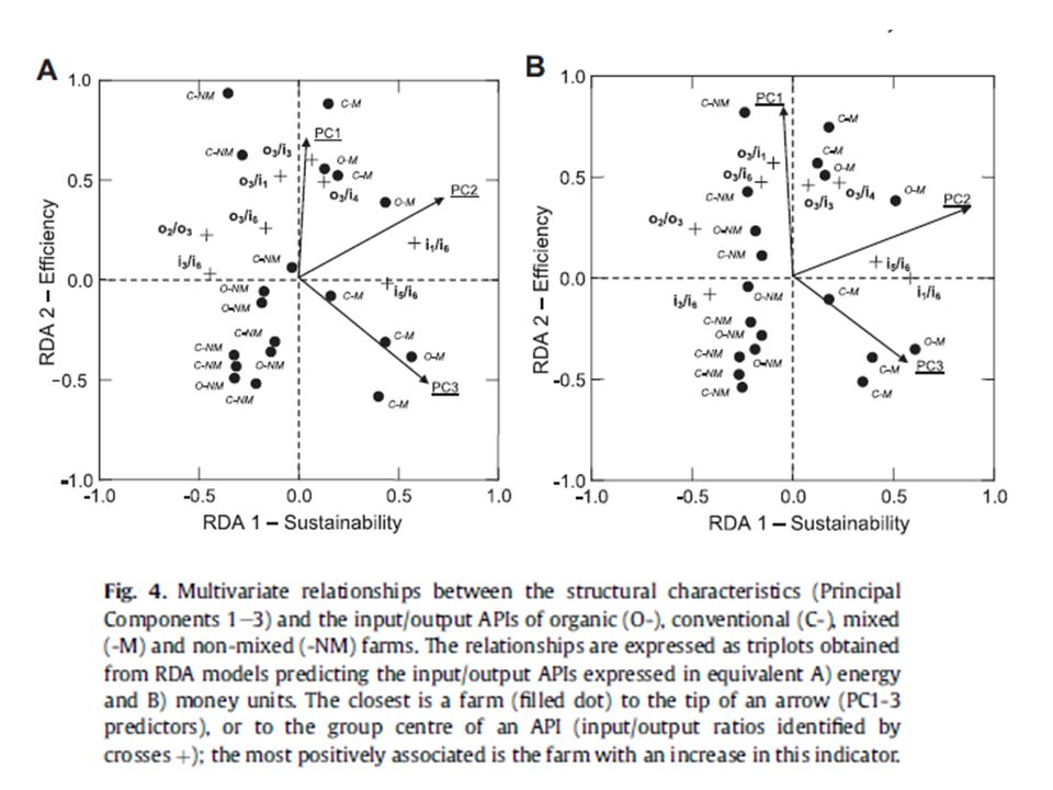
52. Part of Fig 4.

68. What Technique? Response variable(s) ... Predictors(s) No Yes
... is one
• distribution summary
• regression models
... are many
• indirect gradient analysis
(PCA, CA, DCA, MDS)
• cluster analysis
• direct gradient analysis
• constrained cluster analysis
• discriminant analysis (CVA)

69. Raw Data

70. Linear Regression

71. Two Regressions

72. Principal Components

73. Models of Species Response
There are (at least) two models:-
Linear - species increase or decrease along the environmental gradient
Unimodal - species rise to a peak somewhere along the environmental gradient and then fall again

74. Linear

75. Unimodal

76. Ordination Techniques
Linear methods
Weighted averaging (unimodal)
Unconstrained (indirect)
Principal Components
Analysis (PCA)
Correspondence Analysis
(CA)
Constrained (direct)
Redundancy Analysis (RDA)
Canonical
Correspondence Analysis (CCA)

77. Non-metric multidimensional scaling
NMDS maps the observed dissimilarities onto an ordination space by trying to preserve their rank order in a low number of dimensions (often 2) – but the solution is linked to the number of dimensions chosen
it is like a non-linear version of PCO
define a stress function and look for the mapping with minimum stress
(e.g. sum of squared residuals in a monotonic regression of NMDS space distances between original and mapped dissimilarities)
need to use an iterative process, so try with many different starting points and convergence is not guaranteed

78. Procrustes rotation
used to compare graphically two separate ordinations