Download presentation
Presentation is loading. Please wait.

1
Ensemble Data Assimilation Massimo Bonavita ECMWF Acknowledgments: Lars Isaksen, Elias Holm, Mike Fisher, Laure Raynaud

2
Outline The Ensemble Data Assimilation method
What do we do with the EDA? Use of EDA variances in ECMWF 4DVar 4DVar assimilation experiments Conclusions and plans

3
Outline The Ensemble Data Assimilation method
What do we do with the EDA? Use of EDA variances in 4DVar 4DVar assimilation experiments Conclusions and plans

4
The EDA method “When simulating the error evolution of the reference system one should use the reference gain matrix K” (Berre et al. 2007)
 .")
5
The EDA method This is what an ensemble of 4DVar analyses with random observation and SST perturbations does! εa/f/o = perturbations w.r.to ensemble mean Analysis xb+εb y+εo SST+εSST (etc.) xa+εa Forecast xf+εf
 xa+εa. Forecast. xf+εf.")
6
The EDA method After a few cycles the EDA system will have forgotten the initial background perturbations We are diagnosing the background error statistics of the actual analysis system However: We assume that observation and SST errors are correctly specified We need to account for the model error component of the background error

7
The EDA method from: Lars Isaksen
“Stochastic Kinetic Energy Backscatter” SKEB (Berner et al., 2009) ΔXperturbed physics= f(KE,ΔXphysics,n) A fraction of the dissipated energy is backscattered upscale and acts as stream function forcing on resolved-scale flow. Spectral Markov chain: temporal and spatial correlations prescribed Only vorticity perturbed, so only wind field directly affected All levels are perturbed. Either randomly or partially correlated. “Stochastically Perturbed Parameterisation Tendencies” SPPT (Leutbecher, 2009) ΔXperturbed physics= ( 1+μr) ΔXphysics Random pattern r varies smoothly in space and time, with de-correlation scales 500 km and 6 hours. Gaussian distribution with no bias and stdev 0.5 (limited to ±3stdev) Same random number r for X=T, q, u, v No perturbations in lowest 300 m and above 50 hPa (0≤ μ ≤1). from: Lars Isaksen
 ΔXperturbed physics= f(KE,ΔXphysics,n) A fraction of the dissipated energy is backscattered upscale and acts as stream function forcing on resolved-scale flow. Spectral Markov chain: temporal and spatial correlations prescribed. Only vorticity perturbed, so only wind field directly affected. All levels are perturbed. Either randomly or partially correlated. Stochastically Perturbed Parameterisation Tendencies SPPT (Leutbecher, 2009) ΔXperturbed physics= ( 1+μr) ΔXphysics. Random pattern r varies smoothly in space and time, with de-correlation scales 500 km and 6 hours. Gaussian distribution with no bias and stdev 0.5 (limited to ±3stdev) Same random number r. for X=T, q, u, v. No perturbations in lowest 300 m and above 50 hPa (0≤ μ ≤1). from: Lars Isaksen.")
8
The EDA method Comparing the impact of various stochastic perturbation methods: zonal mean u wind ensemble background forecast spread from: Lars Isaksen N S Impact of SKEB on U spread Additional Impact of SPPT on U spread

9
The EDA method Comparing the impact of various stochastic perturbation methods: zonal mean Temperature ensemble background forecast spread from: Lars Isaksen N S Impact of SKEB on T spread Additional Impact of SPPT on T spread

10
The EDA method In the EDA context model error parametrizations should increase spread where/when errors are larger => should increase spread-error correlation Are they doing this?

11
The EDA method EDA (baseline) - EDA+SKEB EDA+SPPT - EDA+SPPT+SKEB
 - EDA+SKEB EDA+SPPT - EDA+SPPT+SKEB")
12
The EDA method EDA (baseline) - EDA+SKEB EDA+SPPT - EDA+SPPT+SKEB
 - EDA+SKEB EDA+SPPT - EDA+SPPT+SKEB")
13
The EDA method Model error parametrizations do increase spread-error correlations Large effect in the lower troposphere Tropics Small effect in the Extratropics Similar behaviour-performance of the two schemes and their combination

14
The EDA method 10 ensemble members using 4D-Var assimilations
T399 outer loop, T95/T159 inner loop (reduced number of iterations) Observations randomly perturbed Cloud track wind (AMV) correlations taken into account SST perturbed with realistically scaled structures Model error represented by stochastic methods (SPPT, Leutbecher, 2009) All 107 conventional and satellite observations used from: Lars Isaksen
 Observations randomly perturbed. Cloud track wind (AMV) correlations taken into account. SST perturbed with realistically scaled structures. Model error represented by stochastic methods (SPPT, Leutbecher, 2009) All 107 conventional and satellite observations used. from: Lars Isaksen.")
15
Outline The Ensemble Data Assimilation method
What do we do with the EDA? Use of EDA variances in ECMWF 4DVar 4DVar assimilation experiments Conclusions and plans

16
What do we do with the EDA?
The EDA simulates the error evolution of the 4DVar analysis cycle. As such it can be applied to: Compute climatology of B matrix for use at the initial time of 4DVar (Analysis-Ensemble method, Fisher 2003; see talk on B matrix modelling) Provide initial conditions for ensemble forecasts (EPS) Provide a flow-dependent sample of background errors at the initial time of 4DVar
 Provide initial conditions for ensemble forecasts (EPS) Provide a flow-dependent sample of background errors at the initial time of 4DVar.")
17
What do we do with the EDA?
Improving Ensemble Prediction System by including EDA perturbations for initial uncertainty The Ensemble Prediction System (EPS) benefits from using EDA based perturbations. Replacing evolved singular vector perturbations by EDA based perturbations improve EPS spread, especially in the tropics. The Ensemble Mean has slightly lower error when EDA is used. N.-Hem. Tropics EVO-SVINI EDA-SVINI EVO-SVINI EDA-SVINI Ensemble spread and Ensemble mean RMSE for 850hPa T
 benefits from using EDA based. perturbations. Replacing evolved singular vector perturbations by EDA. based perturbations improve EPS spread, especially in the tropics. The Ensemble Mean has slightly lower error when EDA is used. N.-Hem. Tropics. EVO-SVINI. EDA-SVINI. EVO-SVINI. EDA-SVINI. Ensemble spread and Ensemble mean RMSE for 850hPa T.")
18
What do we do with the EDA?
The EDA simulates the error evolution of the 4DVar analysis cycle. As such it can be applied to: Compute climatology of B matrix for use at the initial time of 4DVar (Analysis-Ensemble method, see talk on B matrix modelling) Provide initial conditions for ensemble forecasts (EPS) Provide a flow-dependent sample of background errors at the initial time of 4DVar
 Provide initial conditions for ensemble forecasts (EPS) Provide a flow-dependent sample of background errors at the initial time of 4DVar.")
19
What do we do with the EDA?
4DVAr does not cycle error information (B), only the state estimate 4DVar behaves like a Kalman filter in which the covariance matrix is reset to some static matrix B every few hours (12h in ECMWF implement.) Two possible ways around this: Run 4DVar over a long enough window so that the influence of the initial state and errors on the final state analysis is negligible
, only the state estimate. 4DVar behaves like a Kalman filter in which the covariance matrix is reset to some static matrix B every few hours (12h in ECMWF implement.) Two possible ways around this: Run 4DVar over a long enough window so that the influence of the initial state and errors on the final state analysis is negligible.")
20
Memory of the initial state disappears after approx. 3 days
Analysis experiment started with satellite data reintroduced on 15th August 2005 Memory of the initial state disappears after approx. 3 days From Mike Fisher

21
What do we do with the EDA?
An analysis window of ≥3 days would allow 4DVar analysis at final time to be independent of initial state and error estimates However: An effective model error representation must be applied to reconcile model and measurements over a long analysis time window (i.e., weak constraint 4DVar) We would still lack an estimate of analysis errors
 We would still lack an estimate of analysis errors.")
22
What do we do with the EDA?
Two possible ways around this: Run 4DVar over a long enough window so that the influence of the initial state and errors on the final state analysis is negligible Use a sequential method (EDA, EnKF) to cycle error covariance information
 to cycle error covariance information.")
23
Hybrid methods Use of ensemble perturbations in a 3-4DVar analysis
µεσον τε και αριστον Aristotle, Nic. Ethics 2.6 Hybrid methods Use of ensemble perturbations in a 3-4DVar analysis Cycle error information through ensemble of Data Assimilations Retain the implicit full rank error representation of 3-4DVar

24
What do we do with the EDA?
Hybrid systems Ensemble perturbations can be used in a 3-4DVar analysis in a number of different ways: Use ensemble variances for observation QC Use ensemble (co)variances as starting B matrix of minimization (often in linear combination with climatological B, extra control variable) Use of ensemble covariances inside 4DVar minimization (En4DVAR)
variances as starting B matrix of minimization (often in linear combination with climatological B, extra control variable) Use of ensemble covariances inside 4DVar minimization (En4DVAR)")
25
Outline The Ensemble Data Assimilation method
What do we do with the EDA? Use of EDA variances in ECMWF 4DVar 4DVar assimilation experiments Conclusions and plans

26
Use of EDA variances in 4DVar
We want to use EDA perturbations to simulate 4DVar flow-dependent error covariance evolution We start with the diagonal of the Pf matrix, i.e.: “Estimate the first guess error variances with the variance of the EDA short range forecasts” This has been tried before (Kucukkaraca and Fisher, 2006, Fisher 2007, Isaksen et al., 2007) but results have been inconclusive
 but results have been inconclusive.")
27
Use of EDA variances in 4DVar
Define: Veda = EDA sampled variance V* = True error variance Then the estimation error can be decomposed: Veda-V* = E[Veda-V*] + (Veda-E[Veda]) systematic random Similarly for mean square of the estimation error: E[(Veda-V*)2] = (E[Veda-V*])2 + E[(Veda-E[Veda])2] systematic random We should try to minimize both!
 systematic random. Similarly for mean square of the estimation error: E[(Veda-V*)2] = (E[Veda-V*])2 + E[(Veda-E[Veda])2] systematic random. We should try to minimize both!")
28
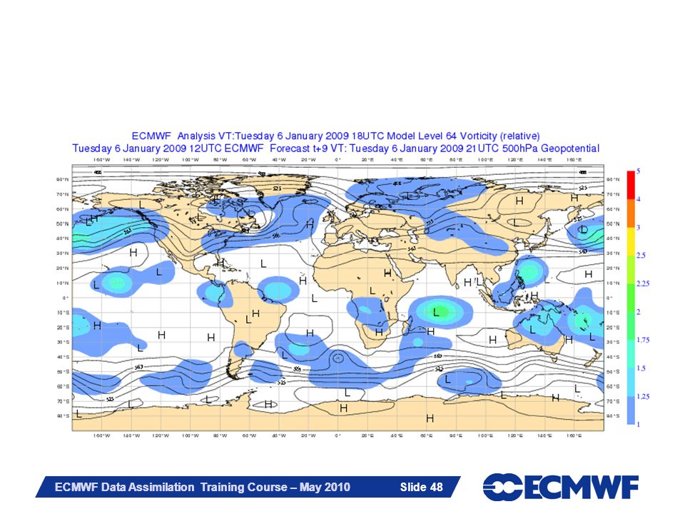
Use of EDA variances in 4DVar
What raw ensemble variances look like? Spread of Vorticity FG t+9h ml=64

29
Use of EDA variances in 4DVar
Noise level is due to sampling errors: 10 member ensemble EDA is a stochastic system: variance of variance estimator ~ 1/Nens We need a system to effectively filter out noise from first guess ensemble forecast variances: Reduce the random component of the estimation error

30
Use of EDA variances in 4DVar
“Mallat et al.: 1998, Annals of Statistics, 26,1-47” Define Ge(i) as the random component of the sampling error in the estimated ensemble variance at gridpoint i: Then the covariance of the sampling noise can be shown to be a simple function of the expectation of the ensemble-based covariance matrix: (1)
 as the random component of the sampling. error in the estimated ensemble variance at gridpoint. i: Then the covariance of the sampling noise can be. shown to be a simple function of the. expectation of the ensemble-based covariance matrix: (1)")
31
Use of EDA variances in 4DVar
“Mallat et al.: 1998, Annals of Statistics, 26,1-47” A consequence of (1) is that: (2) i.e., sampling noise is smaller scale than background error. If the variance field varies on larger scales then the background error => we can use a spectral filter to disentangle noise error from the sampled variance field
 is that: (2) i.e., sampling noise is smaller scale than background. error. If the variance field varies on larger scales then the. background error. => we can use a spectral filter to disentangle noise error. from the sampled variance field.")
32
Use of EDA variances in 4DVar

33
Use of EDA variances in 4DVar
There is indeed a scale separation between signal and sampling noise! Truncation wavenumber is determined by maximizing signal-to-noise ratio of filtered variances (details in Raynaud et al., 2009, and forthcoming Tech. Memo) Optimal truncation wavenumber depends on parameter and model level
 Optimal truncation wavenumber depends on parameter and model level.")
34
Use of EDA variances in 4DVar
Raw Ensemble StDev VO ml64 Filtered Ensemble StDev VO ml64

35
Use of EDA variances in 4DVar
Raw Ensemble StDev Spec. Hum. ml64 Filtered Ensemble StDev Spec. Hum. ml64

36
Use of EDA variances in 4DVar
Operational StDev Random. Method (Fisher & Courtier, 1995 Filtered Ensemble StDev VO ml64

37
Use of EDA variances in 4DVar
Is Filtering the Ensemble Variances enough to improve the analysis? Not quite… N.Hem. Z 500hPA AC S.Hem. Z 500hPA AC

38
Use of EDA variances in 4DVar
Should we also do something about the systematic component of the estimation error? E[(Veda-V*)2] = (E[Veda-V*])2 + E[(Veda-[Veda])2] systematic random A statistically reliable ensemble satisfies:
2] = (E[Veda-V*])2 + E[(Veda-[Veda])2] systematic random. A statistically reliable ensemble satisfies:")
39
Use of EDA variances in 4DVar
Vorticity ml 30 (~50hPa) Ensemble Error Ensemble Spread Spread - Error
 Ensemble Error Ensemble Spread. Spread - Error.")
40
Use of EDA variances in 4DVar
Vorticity ml 78 (~850hPa) Ensemble Error Ensemble Spread Spread - Error
 Ensemble Error Ensemble Spread. Spread - Error.")
41
Use of EDA variances in 4DVar
Is the ensemble fg statistically calibrated? Calibration factors needs to be model level, latitude and parameter dependent Calibration factors seems also to be flow-dependent, i.e. depend on the size of the expected error

42
Use of EDA variances in 4DVar

43
Use of EDA variances in 4DVar
Calibration factors need to be flow-dependent, too! Do they also change in time?

44
Use of EDA variances in 4DVar

45
Use of EDA variances in 4DVar

46
Use of EDA variances in 4DVar
There is not a large day-to-day variability but seasonal variability is important General solution: slowly varying adaptive calibration coefficients

47
Variance Recalibration
EDA Cycle xa+εia Analysis Forecast SST+εiSST y+εio xb+εib xf+εif i=1,2,…,10 Variance post-process εif raw variances Variance Recalibration Variance Filtering EDA scaled variances 4DVar Cycle xa Analysis Forecast EDA scaled Var xb xf

49
Outline The Ensemble Data Assimilation method
What do we do with the EDA? Use of EDA variances in ECMWF 4DVar 4DVar assimilation experiments Conclusions and plans

50
4DVar assimilation with EDA variances
Deterministic DA experiments with EDA variances CY35r3_esuite, T799L91, 7/01 – 16/ Control f8a4 Experiment fb4k with ensemble DA variances: Calibration step: adaptive, flow-dependent, regionally varying, for each parameter and model level Filtering step: “Optimal” spectral filtering EDA variances are used both in observation QC and start of 4DVar minimization

51
4DVar assimilation with EDA variances

52
4DVar assimilation with EDA variances
N.HEM Z ac Jan-Feb

53
4DVar assimilation with EDA variances
S.HEM Z ac Jan-Feb

54
4DVar assimilation with EDA variances
TROP. VW RMSE Jan-Feb

55
4DVar assimilation with EDA variances
Deterministic DA experiments with EDA variances CY36r2_esuite, T1279L91, 7/08 – 16/ Control far9 Experiment fb9x with ensemble DA variances: Calibration step: adaptive, flow-dependent, regionally varying, for each parameter and model level Filtering step: “Optimal” spectral filtering EDA variances are used both in observation QC and start of 4DVar minimization

56
4DVar assimilation with EDA variances
N.HEM Z ac Aug-Sep

57
4DVar assimilation with EDA variances
S.HEM Z ac Aug-Sep

58
4DVar assimilation with EDA variances
TROP VW RMSE Aug-Sep

59
4DVar assimilation with EDA variances
Deterministic DA experiments with EDA variances Results are generally positive in the Extra-Tropics (more so in the NH) Small positive impact in the Tropics
 Small positive impact in the Tropics.")
60
4DVar assimilation with EDA variances
Observation departures statistics support the idea that (slightly) different observation usage is the result of smarter OBS QC decisions
 different observation usage is the result of smarter OBS QC decisions.")
61
Outline The Ensemble Data Assimilation method
What do we do with the EDA? Use of EDA variances in ECMWF 4DVar 4DVar assimilation experiments Conclusions and plans

62
Conclusions and plans First step towards an error cycling DA
Use of flow dependent EDA variances has the potential to improve the deterministic scores A careful post-processing step of the raw ensemble first guess forecast is necessary to: Filter sampling noise Adaptively calibrate the ensemble

63
Conclusions and plans Better OBS QC decisions seems to be playing a part Further improvements in model error parameterizations will directly benefit the system Increase in ensemble size will benefit the system

64
Conclusions and plans WHERE NEXT
Operational implementation and testing Further tuning of system at full operational resolution (T1279L91)
")
65
Conclusions and plans Generalize the use of EDA variances to unbalanced components of control vector Relax the assumption: analysis=“truth” in the calibration step

66
Conclusions and plans Medium term:
Refine the representation of initial uncertainties (correlated perturbations, surface fields uncertainties) in stochastic EDA Evaluate EnKF covariances Further develop the hybridization of 4DVar with EDA (investigate the use of EDA covariances)
 in stochastic EDA. Evaluate EnKF covariances. Further develop the hybridization of 4DVar with EDA (investigate the use of EDA covariances)")
67
Thanks for your attention!
I welcome your questions/comments…

Similar presentations


>")


