Download presentation
Presentation is loading. Please wait.

1
} Chapter 2. Grain Texture
Clastic sediment and sedimentary rocks are made up of discrete particles. The texture of a sediment refers to the group of properties that describe the individual and bulk characteristics of the particles making up a sediment: Individual Grain Size Bulk (Grain Size Distribution) Grain Shape Grain Orientation } Secondary properties that are related to the others. Porosity Permeability
 Grain Shape. Grain Orientation. } Secondary properties. that are related to the. others. Porosity. Permeability.")
2
These properties collectively make up the texture of a sediment or sedimentary rock.
Each can be used to infer something of: The history of a sediment. The processes that acted during transport and deposition of a sediment. The behavior of a sediment. This section focuses on each of these properties, including: Methods of determining the properties. The terminology used to describe the properties. The significance of the properties.

3
Grain Size I. Grain Volume (V) a) Based on the weight of the particle: Where: m is the mass of the particle. V is the volume of the particle. rs is the density of the material making up the particle. (r is the lower case Greek letter rho). 1. Weigh the particle to determine m. 2. Determine or assume a density. (density of quartz = 2650kg/m3) 3. Solve for V. Error due to error in assumed density; Porous material will have a smaller density and less solid volume so this method will underestimate the overall volume.
. 1. Weigh the particle to determine m. 2. Determine or assume a density. (density of quartz = 2650kg/m3) 3. Solve for V. Error due to error in assumed density; Porous material will have a smaller density and less solid volume so this method will underestimate the overall volume.")
4
b) Direct measurement by displacement.
 Direct measurement by displacement.")
5
b) Direct measurement by displacement.
 Direct measurement by displacement.")
6
b) Direct measurement by displacement.
 Direct measurement by displacement.")
7
Accuracy depends on how accurately the displaced volume can be measured.
Not practical for very small grains. For porous materials this method will underestimate the external volume of the particle.

8
c) Based on dimensions of the particle.
Where: d is the diameter of the particle And the particle is a perfect sphere. Measure the diameter of the particle and solve for V. Problem: natural particles are rarely spheres.

9
II. Linear dimensions. a) Direct Measurement Natural particles normally have irregular shapes so that it is difficult to determine what linear dimensions should be measured. Most particles are not spheres so we normally assume that they can be described as triaxial ellipsoids that are described in terms of three principle axes: dL or a-axis longest dimension. dI or b-axis intermediate dimension. dS or c-axis shortest dimension.

10
To define the three dimensions requires a systematic method so that results by different workers will be consistent. Sedimentologists normally use the Maximum Tangent Rectangle Method. Step 1. Determine the plane of maximum projection for the particle. -an imaginary plane passing through the particle which is in contact with the largest surface area of the particle. The maximum projection area is the area of intersection of the plane with the particle.

11
Step 2. Determine the maximum tangent rectangle for the maximum projection area.
-a rectangle with sides having maximum tangential contact with the perimeter of the maximum projection area (the outline of the particle) maximum tangent rectangle
 maximum. tangent. rectangle.")
12
Step 2. Determine the maximum tangent rectangle for the maximum projection area.
-a rectangle with sides having maximum tangential contact with the perimeter of the maximum projection area (the outline of the particle) dL is the length of the rectangle. dI is the width of the rectangle.
 dL is the length of the rectangle. dI is the width of the rectangle.")
13
Step 3. Rotate the particle so that you view the surface that is at right angles to the plane of maximum projection. dS is the longest distance through the particle in the direction normal to the plane of maximum projection.

14
The volume of a triaxial ellipsoid is given by:
dL x dI x dS V = 6

15
For fine particles only dL and dI can be measured in thin sections.
Thin sections are 30 micron (30/1000 mm) thick slices of rock through which light can be transmitted. Click here to see how a thin section is made.
 thick slices of rock through which light can be transmitted. Click here to see how a thin section is made.")
16
Axes lengths measured in thin section are “apparent dimensions” of the particle.
The length measured in thin section depends on where in the particle that the plane of the thin section passes.

17
Axes lengths measured in thin section are “apparent dimensions” of the particle.
The length measured in thin section depends on where in the particle that the plane of the thin section passes.

18
Axes lengths measured in thin section are “apparent dimensions” of the particle.
The length measured in thin section depends on where in the particle that the plane of the thin section passes. For a spherical particle its true diameter is only seen in thin section when the plane of the thin section passes through the centre of the particle.

19
The three axes lengths that are commonly measured are often expressed as a single dimension known as the nominal diameter of a particle (dn): dn is the diameter of the sphere with volume (V1) equal the volume (V2) of the particle with axes lengths dL, dI and dS. V1 = volume of the sphere. V2 = volume of a particle. (a triaxial ellipsoid) By the definition of nominal diameter, V1 = V2 Therefore:
 equal the volume (V2) of the particle with axes lengths dL, dI and dS. V1 = volume of the sphere. V2 = volume of a particle. (a triaxial ellipsoid) By the definition of nominal diameter, V1 = V2. Therefore:")
20
dn can be solved by rearranging the terms:

21
dn can be solved by rearranging the terms:

22
dn can be solved by rearranging the terms:

23
dn can be solved by rearranging the terms:
Therefore: Nominal diameter

24
b) Sieving A sample is passed through a vertically stacked set of square-holed screens (sieves). Used to determine the grain size distribution (a bulk property of a sediment).
.")
25
A set of screens are stacked, largest holes on top, smallest on the bottom
and shaken in a sieve shaker (Rotap shakers are recommended). Grains that are larger than the holes remain on a screen and the smaller grains pass through, collecting on the screen with holes just smaller than the grains. The grains collected on each screen are weighed to determine the weight of sediment in a given range of size. The later section on grain size distributions will explain the method more clearly. Details of the sieving method are given in Appendix I of the course notes.
. Grains that are larger than the holes remain on a screen and the smaller grains pass through, collecting on the screen with holes just smaller than the grains. The grains collected on each screen are weighed to determine the weight of sediment in a given range of size. The later section on grain size distributions will explain the method more clearly. Details of the sieving method are given in Appendix I of the course notes.")
26
III. Settling Velocity Another expression of the grain size of a sediment is the settling velocity of the particles. Settling velocity (w; the lower case Greek letter omega ): the terminal velocity at which a particles falls through a vertical column of still water. Possibly a particularly meaningful expression of grain size as many sediments are deposited from water. When a particle is dropped into a column of fluid it immediately accelerates to some velocity and continues falling through the fluid at that velocity (often termed the terminal settling velocity).
: the terminal velocity at which a particles falls through a vertical column of still water. Possibly a particularly meaningful expression of grain size as many sediments are deposited from water. When a particle is dropped into a column of fluid it immediately accelerates to some velocity and continues falling through the fluid at that velocity (often termed the terminal settling velocity).")
27
The speed of the terminal settling velocity of a particle depends on properties of both the fluid and the particle: Properties of the particle include: The size if the particle (d). The density of the material making up the particle (rs). The shape of the particle.
. The density of the material making up the particle (rs). The shape of the particle.")
28
a) Direct measurement Settling velocity can be measured using settling tubes: a transparent tube filled with still water. In a very simple settling tube: A particle is allowed to fall from the top of a column of fluid, starting at time t1. The particle accelerates to its terminal velocity and falls over a vertical distance, L, arriving there at a later time, t2. The settling velocity can be determined:

29
A variety of settling tubes have been devised with different means of determining the rate at which particles fall. Some apply to individual particles while others use bulk samples. Important considerations for settling tube design include: i) Tube length: the tube must be long enough so that the length over which the particle initially accelerates is small compared to the total length over which the terminal velocity is measured. Otherwise, settling velocity will be underestimated.
 Tube length: the tube must be long enough so that the length over which the particle initially accelerates is small compared to the total length over which the terminal velocity is measured. Otherwise, settling velocity will be underestimated.")
30
ii) Tube diameter: the diameter of the tube must be at least 5 times the diameter of the largest particle that will be passed through the tube. If the tube is too narrow the particle will be slowed as it settles by the walls of the tube (due to viscous resistance along the wall). iii) In the case of tubes designed to measure bulk samples, sample size must be small enough so that the sample doesn’t settle as a mass of sediment rather than as discrete particles. Large samples also cause the risk of developing turbulence in the column of fluid which will affect the measured settling velocity.
. iii) In the case of tubes designed to measure bulk samples, sample size must be small enough so that the sample doesn’t settle as a mass of sediment rather than as discrete particles. Large samples also cause the risk of developing turbulence in the column of fluid which will affect the measured settling velocity.")
31
b) Estimating settling velocity based on particle dimensions.
Settling velocity can be calculated using a wide variety of formulae that have been developed theoretically and/or experimentally. Stoke’s Law of Settling is a very simple formula to calculate the settling velocity of a sphere of known density, passing through a still fluid. Stoke’s Law is based on a simple balance of forces that act on a particle as it falls through a fluid.

32
FG, the force of gravity acting to make the particle settle downward through the fluid.
FB, the buoyant force which opposes the gravity force, acting upwards. FD, the “drag force” or “viscous force”, the fluid’s resistance to the particles passage through the fluid; also acting upwards. Force (F) = mass (m) X acceleration (A)
 = mass (m) X acceleration (A)")
33
FG depends on the volume and density (rs) of the particle and is given by:
FB is equal to the weight of fluid that is displaced by the particle: Where r is the density of the fluid. FD is known experimentally to vary with the size of the particle, the viscosity of the fluid and the speed at which the particle is traveling through the fluid. Viscosity is a measure of the fluid’s “resistance” to deformation as the particle passes through it. Where m (the lower case Greek letter mu) is the fluid’s dynamic viscosity and U is the velocity of the particle; 3pd is proportional to the area of the particle’s surface over which viscous resistance acts.
 is the fluid’s dynamic viscosity and U is the velocity of the particle; 3pd is proportional to the area of the particle’s surface over which viscous resistance acts.")
34
FG and FB are commonly combined to form the expression for the “submerged weight” ( ) of the particle; the gravity force less the buoyant force: “submerged weight” of the particle. The net gravity force acting on a particle falling through the fluid.

35
We now have two forces acting on the falling particle.
and Acting downward, causing the particle to settle. Acting upward, retarding the settling of the particle. What is the relationship between these two forces at the terminal settling velocity? They are equal: FD =

36
Stoke’s Law is based on this balance of forces.
and Where Such that: The settling velocity can be determined by solving for U, the velocity of the particle, so that U = w. Therefore:

37
Rearranging the terms:
2 Stoke’s Law of Settling

38
Example: A spherical quartz particle with a diameter of 0.1 mm falling through still, distilled water at 20°C d = m rs= 2650kg/m3 r = 998.2kg/m3 m = ´ 10-3 Ns/m2 g = m/s2 Under these conditions (i.e., with the values listed above) Stoke’s Law reduces to: For a m particle: w = ´ 10-3 m/s or » 9 mm/s
 Stoke’s Law reduces to: For a m particle: w = ´ 10-3 m/s or » 9 mm/s.")
39
Stoke’s Law has several limitations:
i) It applies well only to perfect spheres (in deriving Stoke’s Law the volume of spheres was used). The drag force (3pdmw) is derived experimentally only for spheres. Non-spherical particles will experience a different distribution of viscous drag. ii) It applies only to still water. Settling through turbulent waters will alter the rate at which a particle settles; upward-directed turbulence will decrease w whereas downward-directed turbulence will increase w.
 It applies well only to perfect spheres (in deriving Stoke’s Law the volume of spheres was used). The drag force (3pdmw) is derived experimentally only for spheres. Non-spherical particles will experience a different distribution of viscous drag. ii) It applies only to still water. Settling through turbulent waters will alter the rate at which a particle settles; upward-directed turbulence will decrease w whereas downward-directed turbulence will increase w.")
40
iii) It applies to particles 0.1 mm or finer.
 It applies to particles 0.1 mm or finer.")
41
iii) It applies to particles 0.1 mm or finer.
Coarser particles, with larger settling velocities, experience different forms of drag forces. Stoke’s Law overestimates the settling velocity of quartz density particles larger than 0.1 mm.

42
When settling velocity is low (d<0
When settling velocity is low (d<0.1mm) flow around the particle as it falls smoothly follows the form of the sphere. When settling velocity is high (d>0.1mm) flow separates from the sphere and a wake of eddies develops in its lee. Drag forces (FD) are only due to the viscosity of the fluid. Pressure forces acting on the sphere vary. Negative pressure in the lee retards the passage of the particle, adding a new resisting force. Stoke’s Law neglects resistance due to pressure.
 flow around the particle as it falls smoothly follows the form of the sphere. When settling velocity is high (d>0.1mm) flow separates from the sphere and a wake of eddies develops in its lee. Drag forces (FD) are only due to the viscosity of the fluid. Pressure forces acting on the sphere vary. Negative pressure in the lee retards the passage of the particle, adding a new resisting force. Stoke’s Law neglects resistance due to pressure.")
43
iv) Settling velocity is temperature dependant because fluid viscosity and density vary with temperature. Temp m r w °C Ns/m Kg/m3 mm/s ´ ´

44
Grain size is sometimes described as a linear dimension based on Stoke’s Law:
Stoke’s Diameter (dS): the diameter of a sphere with a Stoke’s settling velocity equal to that of the particle. Set d = dS and solve for dS.
: the diameter of a sphere with a Stoke’s settling velocity equal to that of the particle. Set d = dS and solve for dS.")
45
IV. Grade Scales Grade scales define limits to a range of grain sizes for a given class (grade) of grain size. Sedimentologists use the Udden-Wentworth Grade Scale. Sets most boundaries to vary by a factor of 2. They provide a basis for a terminology that describes grain size. e.g., medium sand falls between 0.25 and 0.5 mm.

46
Sedmentologists often express grain size in units call Phi Units (f; the lower case Greek letter phi). Phi units assign whole numbers to the boundaries between size classes. Phi was originally defined as: To make Phi dimensionless it was later defined as: Where dO = 1 mm.

47
Phi is the negative of the power to which 2 is raised such that it equals the dimension in millimetres. 2-0 = 1 2-2 = 0.25 2-3 = 0.125 2-(-6) = 64 With a calculator you can convert millimetres to Phi: You can convert Phi to millimetres:
 = 64. With a calculator you can convert millimetres to Phi: You can convert Phi to millimetres:")
48
Note that when grain size is plotted as phi units grain size becomes smaller towards the right.

49
V. Describing Grain Size Distributions
a) Grain Size Data Data on grain size distributions are normally collected by sieving. 1. Grain Size Class (f) 2. Weight (grams) 3. Weight (%) 4. Cumulative Weight (%) -0.5 0.40 1.3 1.42 4.6 5.9 0.5 2.76 8.9 14.8 1.0 4.92 15.9 30.7 1.5 5.96 19.3 50.0 2.0 69.3 2.5 85.2 3.0 94.1 3.5 98.7 4.0 100 Total: 30.92
 Grain Size Data. Data on grain size distributions are normally collected by sieving. 1. Grain Size Class (f) 2. Weight. (grams) 3. Weight. (%) 4. Cumulative Weight (%) Total:")
50
1. Grain size class: the size of holes on which the weighed sediment was trapped in a stack of sieves. 2. Weight (grams): the weight, in grams, of sediment trapped on the sieve denoted by the grain size class. 1. Grain Size Class (f) 2. Weight (grams) 3. Weight (%) 4. Cumulative Weight (%) -0.5 0.40 1.3 1.42 4.6 5.9 0.5 2.76 8.9 14.8 1.0 4.92 15.9 30.7 1.5 5.96 19.3 50 2.0 69.3 2.5 85.2 3.0 94.1 3.5 98.7 4.0 100 Total: 30.92 3. Weight (%): the weight of sediment trapped expressed as a percentage of the weight of the total sample. 4. Cumulative Weight (%): the sum of the weights expressed as a percentage (column 3).
: the weight, in grams, of sediment trapped on the sieve denoted by the grain size class. 1. Grain Size Class (f) 2. Weight. (grams) 3. Weight. (%) 4. Cumulative Weight (%) Total: Weight (%): the weight of sediment trapped expressed as a percentage of the weight of the total sample. 4. Cumulative Weight (%): the sum of the weights expressed as a percentage (column 3).")
51
Each value in column 4 is the percentage of the sample that is coarser than the screen on which the sediment was trapped. 1. Grain Size Class (f) 2. Weight (grams) 3. Weight (%) 4. Cumulative Weight (%) -0.5 0.40 1.3 1.42 4.6 5.9 0.5 2.76 8.9 14.8 1.0 4.92 15.9 30.7 1.5 5.96 19.3 50 2.0 69.3 2.5 85.2 3.0 94.1 3.5 98.7 4.0 100 Total: 30.92
 2. Weight. (grams) 3. Weight. (%) 4. Cumulative Weight (%) Total:")
52
30.7% of the total sample is coarser than 1.0 f.
Each value in column 4 is the percentage of the sample that is coarser than the screen on which the sediment was trapped. 1. Grain Size Class (f) 2. Weight (grams) 3. Weight (%) 4. Cumulative Weight (%) -0.5 0.40 1.3 1.42 4.6 5.9 0.5 2.76 8.9 14.8 1.0 4.92 15.9 30.7 1.5 5.96 19.3 50 2.0 69.3 2.5 85.2 3.0 94.1 3.5 98.7 4.0 100 Total: 30.92 30.7% of the total sample is coarser than 1.0 f.
 2. Weight. (grams) 3. Weight. (%) 4. Cumulative Weight (%) Total: % of the total sample is coarser than 1.0 f.")
53
30.7% of the total sample is coarser than 1.0 f.
Each value in column 4 is the percentage of the sample that is coarser than the screen on which the sediment was trapped. 1. Grain Size Class (f) 2. Weight (grams) 3. Weight (%) 4. Cumulative Weight (%) -0.5 0.40 1.3 1.42 4.6 5.9 0.5 2.76 8.9 14.8 1.0 4.92 15.9 30.7 1.5 5.96 19.3 50 2.0 69.3 2.5 85.2 3.0 94.1 3.5 98.7 4.0 100 Total: 30.92 30.7% of the total sample is coarser than 1.0 f. 85.2% of the total sample is coarser than 2.5 f.
 2. Weight. (grams) 3. Weight. (%) 4. Cumulative Weight (%) Total: % of the total sample is coarser than 1.0 f. 85.2% of the total sample is coarser than 2.5 f.")
54
b) Displaying Grain Size Data
i) Histograms Readily shows the relative amount of sediment in each size class. Each bar width equals the class interval (0.5 f intervals in this case). Bars extend from the maximum size to the minimum size for each size class.
 Histograms. Readily shows the relative amount of sediment in each size class. Each bar width equals the class interval (0.5 f intervals in this case). Bars extend from the maximum size to the minimum size for each size class.")
55
ii) Frequency Curves A smooth curve that joins the midpoints of each bar on the histogram.
 Frequency Curves A smooth curve that joins the midpoints of each bar on the histogram.")
56
iii) Cumulative Frequency Curves
A smooth curve that represents the size distribution of the sample. Several curves for different samples can be plotted together on one diagram for comparison of the samples.

57
Sedimentologists commonly plot cumulative frequency curves on a probability scale for the cumulative frequency. On such plots normal, bell shaped distributions plot as a straight line.

58
Plots of samples which are made up of normally distributed subpopulations plot as a series of straight line segments, each segment representing a normally distributed subpopulation.

59
Plots of samples which are made up of normally distributed subpopulations plot as a series of straight line segments, each segment representing a normally distributed subpopulation.

60
fn is the grain size that is finer than n% of the total sample.
A benefit of cumulative frequency plots is that percentiles can be taken direction from the graph. fn is the grain size that is finer than n% of the total sample. fn is referred to as the nth percentile of the sample. In the example f20 is 0.86f 0.86f is that grain size that is finer than 20% of the sample. Conversely, 0.86f is coarser than 80% of the sample.

61
c) Describing Grain Size Distributions.
Folk and Ward (1957) introduced the Graphic Method to estimate the various statistical parameters describing a grain size distribution using only percentiles taken from cumulative frequency curves. Median Mean Standard deviation Skewness Kurtosis )
 introduced the Graphic Method to estimate the various statistical parameters describing a grain size distribution using only percentiles taken from cumulative frequency curves. Median. Mean. Standard deviation. Skewness. Kurtosis. )")
62
i) Median (Md) The midpoint of the distribution; the 50th percentile. 50% of the sample is finer than the median and 50% of the sample is coarser than the median. In this example the Median is approximately 0.35f.

63
ii) Mean (M) The arithmetic average of the distribution. If the distribution is purely symmetrical M = Md. The Udden-Wentworth Scale is used to define terms to describe the sediment based on the mean size. Eg., if M = 0.34f, the sample is said to be coarse sand.

64
Example calculation of the Mean:
1. Determine f16, f50and f84

65
f16 = -0.59f Example calculation of the Mean: Mean
1. Determine f16, f50and f84 f16 = -0.59f

66
f16 = -0.59f f50 = 0.35f Example calculation of the Mean: Mean
1. Determine f16, f50and f84 f16 = -0.59f f50 = 0.35f

67
f16 = -0.59f f50 = 0.35f f84 = 1.27f Example calculation of the Mean:
1. Determine f16, f50and f84 f16 = -0.59f f50 = 0.35f f84 = 1.27f

68
f16 = -0.59f f50 = 0.35f f84 = 1.27f Example calculation of the Mean:
1. Determine f16, f50and f84 f16 = -0.59f f50 = 0.35f f84 = 1.27f = 0.34f

69
iii) Standard Deviation (s; lower case Greek letter sigma)
Also referred to as the sorting coefficient or dispersion coefficient of a sediment. The units of sorting are phi units. A measure of how much variation in grain size is present within a sample. 68% of the total weight of sediment in a sample falls within +/- 1 standard deviation of the mean. E.g., M = 0.34f and s = 0.75f 68% of the sample falls in the range from to 1.09f.

70
Sedimentologists use a specific terminology to describe the sorting of a sediment:
Very well sorted 0 < s < 0.35f Well sorted < s < 0.50f Moderately well sorted 0.5 < s < 0.71f Moderately sorted < s < 1.00f Poorly sorted < s < 2.00f Very poorly sorted < s < 4.00f Extremely poorly sorted s > 4.00f

71
Examples of sorting:

72
iv) Skewness (Sk) A measure of the symmetry of the distribution. Values range from –1.0 to +1.0. Sk = 0 Perfectly symmetrical. Md = M

73
Sk > 0 The distribution has more fine particles than a symmetrical distribution would have. The distribution is said to be fine tailed. M is finer than Md

74
Sk < 0 The distribution has more coarse particles than a symmetrical distribution would have. The distribution is said to be coarse tailed. M is coarser than Md

75
Sk > 0.3 strongly fine skewed
Terminology: Sk > 0.3 strongly fine skewed 0.1 < Sk < 0.3 fine skewed -0.1 < Sk < 0.1 near symmetrical -0.3 < Sk < -0.1 coarse skewed Sk < -0.3 strongly coarse skewed

76
v) Kurtosis (K) A measure of the peakedness of the distribution (related to sorting). K > 1 sharp peaked (Leptokurtic) K = 1 normal (Mesokurtic) K < 1 flat peaked (Platykurtic)
 K < 1 flat peaked (Platykurtic)")
77
VI. Implications of Grain Size
Grain size is a fundamental property of any granular material. It influences other fundamental properties. Historically it was hoped that ancient depositional environments could be determined on the basis of grain size and grain size distributions. When drilling wells (oil, gas, water) the most abundant samples are small pieces of rock called “drill chips”.
 the most abundant samples are small pieces of rock called drill chips .")
78
Anatomy of a Rotary Drilling Rig
Drill bit: Boron alloy buttons +/- diamond grit.

79
Anatomy of a Rotary Drilling Rig

80
Mud is pumped through the drill string to the bit; as the mud rises to the surface it carries “drill chips” along with it. Drill Chips: 1 to 5 millimetre diameter pieces of rock. Collected and bagged as the mud brings the chips to the surface. 1 sample bag represents 3 metres of drilled rock.

81
One attempt to distinguish depositional environments on the basis of grain size distribution focused on beach versus river sands. Samples were collected from rivers and beaches (both lake and ocean beaches) and Skewness was plotted against Sorting Coefficient.
 and Skewness was plotted against Sorting Coefficient.")
86
Beaches tend to have sands that are better sorted and with more common coarse tail skewness than river sands. This reflects the difference in processes that act in rivers and beaches. Rivers transport a wide range of grain sizes: large particles move in contact with the bed and large volumes of fine particles are carried in suspension in the current. Their deposits tend to be relatively poorly sorted and rich in fine particles (+ve or fine tailed skewness).
.")
87
Beaches experience repeated swash and backwash of waves running up the beach face.
The repeated action of the currents washes fine sand from the beach (improving its sorting) and leaving larger grains behind (causing coarse tail skewness).
 and leaving larger grains behind (causing coarse tail skewness).")
88
The difference in processes acting on beaches and in rivers results in distinct differences in their grain size distributions. Other attempts to apply this method had limited results. The problem is that grain size distribution can be inherited from the source material that makes up the sediment. If a beach forms on ancient river sediments then the beach deposits will inherit characteristics of river deposits. If a river erodes through ancient beach deposits then its sediment will bear the characteristics of beach sediments.

89
In rivers it has been found that, overall, sorting of a sediment improves with the distance of transport. The longer the distance of transport the greater the opportunity to remove fine material (in suspension) and to leave coarser material behind, reducing the range of grain sizes present (improving the sorting and decreasing the sorting coefficient). From: Gomez, Rosser, Peacock, Hicks and Palmer, 2001, Downstream fining in a rapidly aggrading gravel bed river. Water Resources Research, v. 37, p
 and to leave coarser material behind, reducing the range of grain sizes present (improving the sorting and decreasing the sorting coefficient). From: Gomez, Rosser, Peacock, Hicks and Palmer, 2001, Downstream fining in a rapidly aggrading gravel bed river. Water Resources Research, v. 37, p")
90
Why measure Grain Size? 1. It is a fundamental property of any granular material. 2. It influences a variety of other properties. 3. It gives clues to the history of a sediment (more details later in the course).
.")
91
Grain Shape An individual property (rather than a bulk property) that is as fundamental as grain size. Shape can be described in a variety of ways: Roundness: a description of how angular the edges of a particle are. Sphericity: how closely a particle’s shape resembles a sphere. Form: the overall appearance of a particle. Surface texture: scratches, pits, grooves, etc. on a particle’s surface.

92
I. Roundness Several methods of description; some more practical than others. a) Wadell’s Roundness (RW) Time consuming and very impractical but results are reliable. RW: the ratio of the average radius of curvature of the corners on the surface of a grain to the radius of curvature of the largest circle that can be inscribed within the projection of the particle. Where N is the number of corners. RW approaches 1 for a perfectly round particle.

93
b) Dobson and Fork Roundness (RF)
RF: the ratio of the radius of curvature of a particle’s sharpest corner (r) to the radius of curvature of the largest circle that can be inscribed on the projection of the particle (R). c) Power’s visual comparison chart.
 to the radius of curvature of the largest circle that can be inscribed on the projection of the particle (R). c) Power’s visual comparison chart.")
94
The most commonly used method of determining roundness.
Defines terms for describing roundness. e.g., 0.25 < RW <0.35 is termed sub-angular. Also gives a “shape parameter” (r) which is a logarithmic transformation of RW so that the boundaries between roundness classes are whole numbers.
 which is a logarithmic transformation of RW so that the boundaries between roundness classes are whole numbers.")
95
II. Sphericity A measure of how closely a particle resembles a sphere. Usually denoted by Y, the capital Greek letter psi. A measure of sphericity is useful to determine whether or not Stoke’s Law of settling is applicable (e.g., how much a particle differs from a sphere). Sphericity determines the use of a sediment (e.g., high sphericity sediment is not particularly good for making concrete).
. Sphericity determines the use of a sediment (e.g., high sphericity sediment is not particularly good for making concrete).")
96
a) Wadell’s Sphericity (Y)
Y: the ratio of the diameter of a sphere with the same volume as the particle to the volume diameter of a sphere that will circumscribe the particle. Where VS is the volume of the particle and VC is the volume of the circumscribing sphere. There are a couple of methods of determining Y.

97
Where VS is the volume of the particle and VC is the volume of the circumscribing sphere.
i) Based on volume measurement. Step 1. Measure the volume of the particle by displacement in water in a graduated cylinder. This determines VS. Step 2. Measure the long axis of the particle (dL) as this will be the diameter of the largest circumscribing sphere. By this procedure:
 Based on volume measurement. Step 1. Measure the volume of the particle by displacement in water in a graduated cylinder. This determines VS. Step 2. Measure the long axis of the particle (dL) as this will be the diameter of the largest circumscribing sphere. By this procedure:")
98
Where VS is the volume of the particle and VC is the volume of the circumscribing sphere.
ii) Approximate VS by assuming that the particle is a triaxial ellipsoid. and 2 By either method, as Y approaches 1 the particle approaches a sphere in overall shape (i.e., for a perfect sphere Y = 1).
 Approximate VS by assuming that the particle is a triaxial ellipsoid. and. 2. By either method, as Y approaches 1 the particle approaches a sphere in overall shape (i.e., for a perfect sphere Y = 1).")
99
b) Sneed and Folk (YP) or Maximum Projection Sphericity
YP: the ratio of the maximum projection area of a sphere with volume equal to the particle to the maximum projection area of the particle. Sneed and Folk argued that it was the projection area of a particle that experienced the viscous drag of moving fluid, therefore it was more important than the volume of the particle. With increasing sphericity.

100
c) Corey Shape Factor (SF)
Not really a measure of sphericity but similar to YP. Used in a variety formulae used to calculate sediment transport rates. d) Riley Sphericity (YR) Used when only a two dimensional view is available on thin sections.
 Riley Sphericity (YR) Used when only a two dimensional view is available on thin sections.")
101
III. Form Provides a consistent terminology for describing the overall form of particles. Based on various ratios of dL, dI and dS a) Zingg Form Index Assigns specific shape terms based on ratios of dI/dL and dS/dI. Independent of sphericity although equant particles are highly spherical.
 Zingg Form Index. Assigns specific shape terms based on ratios of dI/dL and dS/dI. Independent of sphericity although equant particles are highly spherical.")
102
b) Sneed and Folk Form Index
Defines 10 shape classes. Shows sphericity for each class.

103
IV. Implications of particle shape
a) Controls on particle shape. i) Lithology For particles that are rock fragments aspects of the lithology of the source rock can influence shape. Massive source rocks (non-bedded) tend to produce more equant particles (e.g., granite, massive sandstone, etc.). Bedded and foliated rocks tend to produce more platy particles (e.g., well-bedded limestones).
 Controls on particle shape. i) Lithology. For particles that are rock fragments aspects of the lithology of the source rock can influence shape. Massive source rocks (non-bedded) tend to produce more equant particles (e.g., granite, massive sandstone, etc.). Bedded and foliated rocks tend to produce more platy particles (e.g., well-bedded limestones).")
104
ii) Hardness Particularly hard clasts (e.g., granite, quartz-cemented sandstone, etc.) change in shape during transport less readily than softer lithologies. Softer lithologies (e.g., limestone) change shape much more readily. Unconsolidated material (e.g., cohesive mud) changes shape almost immediately when it is transported. b) Changes in Shape by Transport Transport of particles by water, wind or flowing glaciers has the potential to cause changes to their shape over time. During transport particles interact with each other and with the surface over which they move. Shape is modified by grinding, chipping and crushing that takes place due to this interaction.
 change in shape during transport less readily than softer lithologies. Softer lithologies (e.g., limestone) change shape much more readily. Unconsolidated material (e.g., cohesive mud) changes shape almost immediately when it is transported. b) Changes in Shape by Transport. Transport of particles by water, wind or flowing glaciers has the potential to cause changes to their shape over time. During transport particles interact with each other and with the surface over which they move. Shape is modified by grinding, chipping and crushing that takes place due to this interaction.")
105
The following figure reports data derived from long distance transport of blocks cut initially as cubes within a circular flume. Changes in roundness and sphericity for cubes of chert (a very hard rock type) and softer limestone. Roundness increases for limestone much more quickly with transport than the harder chert, especially during the early phase of transport.
 and softer limestone. Roundness increases for limestone much more quickly with transport than the harder chert, especially during the early phase of transport.")
106
The rate of increase in roundness is greatest during early transport for both rock types.
As rounding takes place it becomes increasingly more difficult to change the shape to further improve roundness.

107
With an initially angular particle it is relatively easy to increase roundness by breaking off the sharp corners.

108
As the particle becomes rounder, larger and larger masses of material must be removed to cause a comparable increase in roundness.

109
Sphericity changes shape only very slowly because the particles began as relatively equant shaped cubes (i.e., with high sphericity to begin with). Relatively large masses of material must be removed to significantly change the sphericity of a particle. Gray area must be removed to increase sphericity.

110
Gravel size material changes shape relatively rapidly with transport in comparison to sand size material. Shape change in sand can be inferred from rates of change of weight of particles with transport; changes in shape require changes in mass. For quartz grains in the size range 2 mm to 0.05 mm, that are transported in water, the weight loss is <0.1% per 1000 km of transport (the rate is doubled for feldspars). For quartz grains finer than 0.05 mm that are transported in water there is virtually no change in weight with transport.
. For quartz grains finer than 0.05 mm that are transported in water there is virtually no change in weight with transport.")
111
Why so little change in very fine sand?
Breakage takes place during collisions (between grains and a solid substrate) and depends on the amount of momentum that is exchanged during collisions. Momentum = mass ´ velocity Very fine sand, silt and clay particles have very small mass so that they have little momentum. During collisions there is little momentum exchanged and, therefore, little breakage which is required to change the mass and shape of the grains. Momentum is further reduced when transport is in water because the buoyant force reduces its effective weight. Most of the particle’s momentum is used in “pushing” the water as the particle moves, losing momentum due to the viscosity of the water.
 and depends on the amount of momentum that is exchanged during collisions. Momentum = mass ´ velocity. Very fine sand, silt and clay particles have very small mass so that they have little momentum. During collisions there is little momentum exchanged and, therefore, little breakage which is required to change the mass and shape of the grains. Momentum is further reduced when transport is in water because the buoyant force reduces its effective weight. Most of the particle’s momentum is used in pushing the water as the particle moves, losing momentum due to the viscosity of the water.")
112
When transport is in water there is little momentum to cause breakage and change in shape.
Finally, we’ll see later that particles finer than 0.05 mm are transported in suspension (floating in the water column), further reducing the chances of shape-changing collisions. Transport by wind is more effective in changing the shape of fine grains. Air has low density (little buoyant force) and very low viscosity so that there is more momentum exchanged during collisions. Rate of weight loss is 100 to 1000 times that when transport is in water. Eolian desert sands tend to have relatively high sphericity.
, further reducing the chances of shape-changing collisions. Transport by wind is more effective in changing the shape of fine grains. Air has low density (little buoyant force) and very low viscosity so that there is more momentum exchanged during collisions. Rate of weight loss is 100 to 1000 times that when transport is in water. Eolian desert sands tend to have relatively high sphericity.")
113
Shape Sorting by Transport
The roundness and sphericity of particles influence the ease with flowing water can move the particle. To cause an angular cube to roll the fluid force acting on it must overcome the weight of the cube and pivot it 45° before its centre of mass passes over the pivot point. Once the centre of mass passes over the pivot point the weight of the particle aids in the motion.

114
A rounder, octagonal particle need only be pivoted over 20° before it’s center of mass passes over the pivot point and the weight contributes to the motion.

115
For a spherical particle the angle that must be exceeded is very close to 0°.
Overall, the more spherical the particle the more readily it will transported by a moving fluid.

116
“Shape sorting” involves the selective removal of particles due to their shape.
Time 1: angular and spherical particles are introduced to a current. Time 2: the spheres are preferentially removed as they roll away from the site due to the current. The remaining particles are largely angular and the particles down stream are more rounded and spherical.

117
b) Depositional environments and particle shape
Roundness and sphericity may be useful in helping determine ancient environments or processes associated with deposition. Glacial till that is transported within glacial ice is typically angular in shape. Angularity reflects a lack of transport by water prior to deposition. Eolian (windblown) sands commonly have a higher sphericity than water transported sand.
 sands commonly have a higher sphericity than water transported sand.")
118
In rivers changes in roundness and sphericity with transport are well documented.
Demir, 2003, Downstream changes in bed material size and shape characteristics in a small upland stream: Cwm Treweryn, in South Wales, Yerbilimleri, v. 28, p

119
It has been found that, in general, river gravels are relatively compact whereas beach gravels tend to be more platy or disc-shaped.

120
As for grain size distribution, it is the processes in the two environments that differ and lead to the characteristic shapes. In rivers, gravel rolls along the bottom so that more equant or spherical shapes are most commonly transported. On beach faces the swash and backwash may play two rolls in enhancing the enrichment by disc-shaped particles: i) By selectively removing more spherical particles which readily roll down the slope of the beach face, leaving flatter particles behind.
 By selectively removing more spherical particles which readily roll down the slope of the beach face, leaving flatter particles behind.")
121
Problem: lithology plays an important roll in determining shape.
ii) The swash and backwash may lead to back and forth motion of the particle on the beach face. This leads to abrasion of one side and if the waves cause it to flip over abrasion takes place on the other side, ultimately leading to a disc-shaped clast. Time 1 Time 2 Time 3 Time 4 Problem: lithology plays an important roll in determining shape. e.g., a river with a well-bedded limestone source of gravel will have predominantly platy gravel.
 The swash and backwash may lead to back and forth motion of the particle on the beach face. This leads to abrasion of one side and if the waves cause it to flip over abrasion takes place on the other side, ultimately leading to a disc-shaped clast. Time 1. Time 2. Time 3. Time 4. Problem: lithology plays an important roll in determining shape. e.g., a river with a well-bedded limestone source of gravel will have predominantly platy gravel.")
122
Furthermore, like grain size distribution, shape may be inherited from the source material of the particles. A river that erodes through ancient beach gravel will have clasts that are platy in form.

123
Porosity and Permeabilty
Both are important properties that are related to fluids in sediment and sedimentary rocks. Fluids can include: water, hydrocarbons, spilled contaminants. Most aquifers are in sediment or sedimentary rocks. Virtually all hydrocarbons are contained in sedimentary rocks. Porosity: the volume of void space (available to contain fluid or air) in a sediment or sedimentary rock. Permeability: related to how easily a fluid will pass through any granular material.
 in a sediment or sedimentary rock. Permeability: related to how easily a fluid will pass through any granular material.")
124
I. Porosity (P) The proportion of any material that is void space, expressed as a percentage of the total volume of material. Where VP is the total volume of pore space and VT is the total volume of rock or sediment. In practice, porosity is commonly based on measurement of the total grain volume of a granular material: Where VG is the total volume of grains within the total volume of rock or sediment.

125
Porosity varies from 0% to 70% in natural sediments but exceeds 70% for freshly deposited mud.
Several factors control porosity. a) Packing Density Packing density: the arrangement of the particles in the deposit. The more densely packed the particles the lower the porosity. e.g., perfect spheres of uniform size.
 Packing Density. Packing density: the arrangement of the particles in the deposit. The more densely packed the particles the lower the porosity. e.g., perfect spheres of uniform size.")
126
Porosity varies from 0% to 70% in natural sediments but exceeds 70% for freshly deposited mud.
Several factors control porosity. a) Packing Density Packing density: the arrangement of the particles in the deposit. The more densely packed the particles the lower the porosity. e.g., perfect spheres of uniform size. Porosity can vary from 48% to 26%.
 Packing Density. Packing density: the arrangement of the particles in the deposit. The more densely packed the particles the lower the porosity. e.g., perfect spheres of uniform size. Porosity can vary from 48% to 26%.")
127
Shape has an important effect on packing.
Tabular rectangular particles can vary from 0% to just under 50%: Natural particles such as shells can have very high porosity:

128
In general, the greater the angularity of the particles the more open the framework (more open fabric) and the greater the possible porosity. b) Grain Size On its own, grain size has no influence on porosity! d = sphere diameter; n = number of grains along a side (5 in this example). Consider a cube of sediment of perfect spheres with cubic packing.
 Grain Size. On its own, grain size has no influence on porosity! d = sphere diameter; n = number of grains along a side (5 in this example). Consider a cube of sediment of perfect spheres with cubic packing.")
129
Length of a side of the cube = d ´ n = dn
Volume of the cube (VT): Total number of grains: n ´ n ´ n = n3 Volume of a single grain: Total volume of grains (VG):
: Total number of grains: n ´ n ´ n = n3. Volume of a single grain: Total volume of grains (VG):")
130
Where: and Therefore: Rearranging: Therefore: d (grain size) does not affect the porosity so that porosity is independent of grains size. No matter how large or small the spherical grains in cubic packing have a porosity is 48%.

131
There are some indirect relationships between size and porosity.
i) Large grains have higher settling velocities than small grains. When grains settle through a fluid the large grains will impact the substrate with larger momentum, possibly jostling the grains into tighter packing (therefore with lower porosity). ii) A shape effect. Unconsolidated sands tend to decrease in porosity with increasing grain size. Consolidated sands tend to increase in porosity with increasing grain size.
 Large grains have higher settling velocities than small grains. When grains settle through a fluid the large grains will impact the substrate with larger momentum, possibly jostling the grains into tighter packing (therefore with lower porosity). ii) A shape effect. Unconsolidated sands tend to decrease in porosity with increasing grain size. Consolidated sands tend to increase in porosity with increasing grain size.")
132
Generally, unconsolidated sands undergo little burial and less compaction than consolidated sands.
Fine sand has slightly higher porosity. Fine sand tends to be more angular than coarse sand. Therefore fine sand will support a more open framework (higher porosity) than better rounded, more spherical, coarse sand.
 than better rounded, more spherical, coarse sand.")
133
Consolidated sand (deep burial, well compacted) has undergone exposure to the pressure of burial (experiences the weight of overlying sediment). Fine sand is angular, with sharp edges, and the edges will break under the load pressure and become more compacted (more tightly packed with lower porosity). Coarse sand is better rounded and less prone to breakage under load; therefore the porosity is higher than that of fine sand.
. Coarse sand is better rounded and less prone to breakage under load; therefore the porosity is higher than that of fine sand.")
134
c) Sorting In general, the better sorted the sediment the greater the porosity. In well sorted sands fine grains are not available to fill the pore spaces. This figure shows the relationship between sorting and porosity for clay-free sands.

135
Overall porosity decreases with increasing sorting coefficient (poorer sorting).
For clay-free sands the reduction in porosity with increasing sorting coefficient is greater for coarse sand than for fine sand. The difference is unlikely if clay was also available to fill the pores.

136
For clay-free sands the silt and fine sand particles are available to fill the pore space between large grains and reduce porosity.

137
Because clay is absent less relatively fine material is not available to fill the pores of fine sand. Therefore the pores of fine sand will be less well-filled (and have porosity higher).
.")
138
d) Post burial changes in porosity.
Includes processes that reduce and increase porosity. Porosity that develops at the time of deposition is termed primary porosity. Porosity that develops after deposition is termed secondary porosity. Overall, with increasing burial depth the porosity of sediment decreases. 50% reduction in porosity with burial to 6 km depth due to a variety of processes.

139
May include breakage of grains.
i) Compaction Particles are forced into closer packing by the weight of overlying deposits, reducing porosity. May include breakage of grains. Most effective if clay minerals are present (e.g., shale). Freshly deposited mud may have 70% porosity but burial under a kilometre of sediment reduces porosity to 5 or 10%.
 Compaction. Particles are forced into closer packing by the weight of overlying deposits, reducing porosity. May include breakage of grains. Most effective if clay minerals are present (e.g., shale). Freshly deposited mud may have 70% porosity but burial under a kilometre of sediment reduces porosity to 5 or 10%.")
140
ii) Cementation Precipitation of new minerals from pore waters causes cementation of the grains and acts to fill the pore spaces, reducing porosity. Most common cements are calcite and quartz. Here’s a movie of cementation at Paul Heller’s web site.

141
iii) Clay formation Clays may form by the chemical alteration of pre-existing minerals after burial. Feldspars are particularly common clay-forming minerals. Clay minerals are very fine-grained and may accumulate in the pore spaces, reducing porosity. Eocene Whitemud Formation, Saskatchewan

142
iv) Solution If pore waters are undersaturated with respect to the minerals making up a sediment then some volume of mineral material is lost to solution. Calcite, that makes up limestone, is relatively soluble and void spaces that are produced by solution range from the size of individual grains to caverns. Quartz is relatively soluble when pore waters have a low Ph. Solution of grains reduces VG, increasing porosity. Solution is the most effective means of creating secondary porosity. v) Pressure solution The solubility of mineral grains increases under an applied stress (such as burial load) and the process of solution under stress is termed Pressure Solution. The solution takes place at the grain contacts where the applied stress is greatest.
 Pressure solution. The solubility of mineral grains increases under an applied stress (such as burial load) and the process of solution under stress is termed Pressure Solution. The solution takes place at the grain contacts where the applied stress is greatest.")
143
Pressure solution results in a reduction in porosity in two different ways:
1. It shortens the pore spaces as the grains are dissolved. 2. Insoluble material within the grains accumulates in the pore spaces as the grains are dissolve.

144
v) Fracturing Fracturing of existing rocks creates a small increase in porosity. Fracturing is particularly important in producing porosity in rocks with low primary porosity.

145
Why is porosity important?
Especially because it allows us to make estimations of the amount of fluid that can be contained in a rock (water, oil, spilled contaminants, etc.). Example from oil and gas exploration:
. Example from oil and gas exploration:")
146
Why is porosity important?
Especially because it allows us to make estimations of the amount of fluid that can be contained in a rock (water, oil, spilled contaminants, etc.). Example from oil and gas exploration:
. Example from oil and gas exploration:")
147
Why is porosity important?
Especially because it allows us to make estimations of the amount of fluid that can be contained in a rock (water, oil, spilled contaminants, etc.). Example from oil and gas exploration:
. Example from oil and gas exploration:")
148
Why is porosity important?
Especially because it allows us to make estimations of the amount of fluid that can be contained in a rock (water, oil, spilled contaminants, etc.). Example from oil and gas exploration:
. Example from oil and gas exploration:")
149
Why is porosity important?
Especially because it allows us to make estimations of the amount of fluid that can be contained in a rock (water, oil, spilled contaminants, etc.). Example from oil and gas exploration: How much oil is contained in the discovered unit? In this case, assume that the pore spaces of the sediment in the oil-bearing unit are full of oil. Therefore, the total volume of oil is the total volume of pore space (VP) in the oil-bearing unit.
. Example from oil and gas exploration: How much oil is contained in the discovered unit In this case, assume that the pore spaces of the sediment in the oil-bearing unit are full of oil. Therefore, the total volume of oil is the total volume of pore space (VP) in the oil-bearing unit.")
150
Total volume of oil = VP, therefore solve for VP.

151
II. Permeability (Hydraulic Conductivity; k)
Stated qualitatively: permeability is a measure of how easily a fluid will flow through any granular material. More precisely, permeability (k) is an empirically-derived parameter in D’Arcy’s Law, a Law that predicts the discharge of fluid through a granular material.
 is an empirically-derived parameter in D’Arcy’s Law, a Law that predicts the discharge of fluid through a granular material.")
152
D’Arcy’s Law: Another way to express D’Arcy’s Law is as the flow rate as the “apparent velocity” (V) of the fluid through the material where: Thus, D’Arcy’s Law can be expressed as: Expanded:

153
So, the apparent velocity of a fluid flowing through a granular material depends on several factors:
Dp: this is the driving force behind the flow of fluid through granular materials. The greater the change in pressure the greater the rate of flow. (try blowing pop out of a straw!)
")
154
: Apparent velocity decreases with increasing dynamic viscosity.
The higher the viscosity the more difficult it is for the pressure to “push” the fluid through the small pathways within the material. (try sucking molasses through a straw!) : The longer the pathway of the fluid the more pressure is needed to “push” the fluid through the material. (try drinking a milkshake through a 1 metre long straw!) This is a viscous effect: resistance to deformation is cumulative along the length of the tube: the longer the tube (or pathway) the greater the total resistance.
 : The longer the pathway of the fluid the more pressure is needed to. push the fluid through the material. (try drinking a milkshake through a 1 metre long straw!) This is a viscous effect: resistance to deformation is cumulative along the length of the tube: the longer the tube (or pathway) the greater the total resistance.")
155
Those are all properties that are independent of the granular material.
There are also controls on permeability that are exerted by the granular material and are accounted for in the term (k) for permeability: k is proportional to all sediment properties that influence the flow of fluid through any granular material (note that the dimensions of k are cm2). Two major factors: 1. The diameter of the pathways through which the fluid moves. 2. The tortuosity of the pathways (how complex they are).
 for permeability: k is proportional to all sediment properties that influence the flow of fluid through any granular material (note that the dimensions of k are cm2). Two major factors: 1. The diameter of the pathways through which the fluid moves. 2. The tortuosity of the pathways (how complex they are).")
156
1. The diameter of the pathways.
Along the walls of the pathway the velocity is zero (a no slip boundary) and increases away from the boundaries, reaching a maximum towards the middle to the pathway. Narrow pathway: the region where the velocity is low is a relatively large proportion of the total cross-sectional area and average velocity is low. Large pathway: the region where the velocity is low is proportionally small and the average velocity is greater. It’s easier to push fluid through a large Pathway than a small one.
 and increases away from the boundaries, reaching a maximum towards the middle to the pathway. Narrow pathway: the region where the velocity is low is a relatively large proportion of the total cross-sectional area and average velocity is low. Large pathway: the region where the velocity is low is proportionally small and the average velocity is greater. It’s easier to push fluid through a large. Pathway than a small one.")
157
2. The tortuosity of the pathways.
Tortuosity is a measure of how much a pathway deviates from a straight line.

159
2. The tortuosity of the pathways.
Tortuosity is a measure of how much a pathway deviates from a straight line. The path that fluid takes through a granular material is governed by how individual pore spaces are connected. The greater the tortuosity the lower the permeability because viscous resistance is cumulative along the length of the pathway.

160
Pathway diameter and tortuosity are controlled by the properties of the sediment and determine the sediment’s permeability. The units of permeability are Darcies (d): 1 darcy is the permeability that allows a fluid with 1 centipoise viscosity to flow at a rate of 1 cm/s under a pressure gradient of 1 atm/cm. Permeability is often very small and expressed in millidarcies ( )
: 1 darcy is the permeability that allows a fluid with 1 centipoise viscosity to flow at a rate of 1 cm/s under a pressure gradient of 1 atm/cm. Permeability is often very small and expressed in millidarcies ( )")
161
a) Sediment controls on permeability
i) Packing density Tightly packed sediment has smaller pathways than loosely packed sediment (all other factors being equal). Smaller pathways reduce porosity and the size of the pathways so the more tightly packed the sediment the lower the permeability.
 Packing density. Tightly packed sediment has smaller pathways than loosely packed sediment (all other factors being equal). Smaller pathways reduce porosity and the size of the pathways so the more tightly packed the sediment the lower the permeability.")
162
ii) Porosity In general, permeability increases with primary porosity. The larger and more abundant the pore spaces the greater the permeability. Pore spaces must be well connected to enhance permeability.

163
Shale, chalk and vuggy rocks (rocks with large solution holes) may have very high porosity but the pores are not well linked. The discontinuous pathways result in low permeability. Fractures can greatly enhance permeability but do not increase porosity significantly. A 0.25 mm fracture will pass fluid at the rate that would be passed by13.5 metres of rock with 100 md permeability.

164
iii) Grain Size Unlike porosity, permeability increases with grain size. The larger the grain size the larger the pore area. For spherical grains in cubic packing: Pore area = 0.74d2

165
A ten-fold increase in grain size yields a hundred-fold increase in permeability.
iv) Sorting The better sorted a sediment is the greater its permeability. In very well sorted sands the pore spaces are open. In poorly sorted sands fine grains occupy the pore spaces between coarser grains.
 Sorting. The better sorted a sediment is the greater its permeability. In very well sorted sands the pore spaces are open. In poorly sorted sands fine grains occupy the pore spaces between coarser grains.")
166
v) Post-burial processes
Like porosity, permeability is changed following burial of a sediment. In this example permeability is reduced by two orders of magnitude with 3 km of burial. Cementation Clay formation Compaction Pressure solution All act to reduce permeability

167
b) Directional permeability
Permeability is not necessarily isotropic (equal in all directions) Fractures are commonly aligned in the same direction, greatly enhancing permeability in the direction that is parallel to the fractures.
 Fractures are commonly aligned in the same direction, greatly enhancing permeability in the direction that is parallel to the fractures.")
168
Variation in grain size and geological structure can create directional permeability.
E.g., Graded bedding: grain size becomes finer upwards in a bed. Fluid that is introduced at the surface will follow a path that is towards the direction of dip of the beds.

169
Fabric (preferred orientation of the grains in a sediment) can cause directional permeability.
E.g., A sandstone unit of prolate particles. The direction along the long axes of grains will have larger pathways and therefore greater permeability than the direction that is parallel to the long axes.

170
Grain Orientation Fabric: the group of properties that are related to the spatial arrangement of the particles (including packing and orientation). The term is commonly used to refer to orientation only. Why is it important? 1. It can affect other properties. e.g., permeability, how it breaks (building stone). 2. It can have genetic significance. The problem with grain size and shape was that they may be inherited from their source rock.
. 2. It can have genetic significance. The problem with grain size and shape was that they may be inherited from their source rock.")
171
Particle orientation is achieved at the time of deposition in response to processes that acted in the environmental setting. It remains fixed unless: It becomes compacted (the change is trivial for sands). It is structurally deformed (normally such deformation is obvious). It is bioturbated (reworking by organisms that may or may not leave a visible structure).
. It is structurally deformed (normally such deformation is obvious). It is bioturbated (reworking by organisms that may or may not leave a visible structure).")
172
a) How grain orientation is measured.
i) Gravel-size material. Measured in terms of the a-axis (dL), the b-axis (dI) and the plane of maximum projection (the a-b plane). Measure the strike and dip of the a-b plane. Strike will be the trend of the a-axis or the b-axis. Dip is measured from the plane of bedding (not the horizontal plane if the beds are tilted). In tilted rocks measure the dip with respect to the horizontal and correct for regional dip of bedding. The particle will dip along the a- or b-axes.
 Gravel-size material. Measured in terms of the a-axis (dL), the b-axis (dI) and the plane of maximum projection (the a-b plane). Measure the strike and dip of the a-b plane. Strike will be the trend of the a-axis or the b-axis. Dip is measured from the plane of bedding (not the horizontal plane if the beds are tilted). In tilted rocks measure the dip. with respect to the horizontal and correct for regional dip of bedding. The particle will dip along the a- or b-axes.")
173
The dip of a particle is termed imbrication.
The direction is the imbrication direction and the dip angle is the angle of imbrication. On average, the a-axis is either parallel to or perpendicular to the direction of imbrication. Particles that are deposited from water normally dip into the current; imbrication direction is at 180° to the flow of the depositing current.

174
ii) Sand-size material
Can be determined with a microscope from thin sections cut from oriented specimens. Before removing the specimen from the outcrop it should be marked to show: 1. The direction to magnetic north.

175
ii) Sand-size material
Can be determined with a microscope from thin sections cut for oriented specimens. Before removing the specimen from the outcrop it should be marked to show: 1. The direction to magnetic north. 2. The top direction in outcrop.

176
ii) Sand-size material
Can be determined with a microscope from thin sections cut for oriented specimens. Before removing the specimen from the outcrop it should be marked to show: 1. The direction to magnetic north. 2. The top direction in outcrop. 3. The attitude of associated bedding.

177
In the lab, three thin sections must be cut:
1. Parallel to bedding. Determine the orientation of the apparent long axes; this indicates the orientation of the remaining two thin sections. 2. Parallel to the average long axis orientation but perpendicular to bedding. 3. At right angles to the average long axis orientation and perpendicular to bedding. The thin sections allow the identification of the average a-axis orientation, whether the a- or b-axes are imbricate and the direction of imbrication.

178
b) Types of Grain Frabric
i) Isotropic fabric: No preferred alignment of the particles. If the particles are highly spherical no preferred fabric will be discernable. Particles are non-spherical but have no preferred fabric.
 Isotropic fabric: No preferred alignment of the particles. If the particles are highly spherical no preferred fabric will be discernable. Particles are non-spherical but have no preferred fabric.")
179
ii) Anisotropic fabric:
A-axes transverse to flow with b-axes imbricate. a(t)b(i) A-axes parallel to flow with a-axes imbricate. a(p)a(i) Complex fabrics also develop with a mix of a(t)b(i) and a(p)a(i) that may appear isotropic.
b(i) A-axes parallel to flow with a-axes imbricate. a(p)a(i) Complex fabrics also develop with a mix of a(t)b(i) and a(p)a(i) that may appear isotropic.")
180
A problem with measuring grain orientation in thin section:
Like apparent grain size, the orientation that is seen in thin section varies with where the thin section cuts through the grain. Care must be taken to ensure that the thin section is in the plane of bedding and not at a high angle to it.

181
a) Displaying directional data.
Directional data come in a variety of forms including the examples listed below: Particle a-axis orientation; Imbrication direction; Cross-bed dip direction; Symmetrical ripple crest orientation; Orientation of fossils; Sedimentologists normally display such data on circular histograms called “rose diagrams”.

182
The histogram, below, shows the distribution of directional data relatively clearly.
The data shown below appear to be bimodal (one from 0 to 30° and one from 330 to 360°). A single mode (at 120 to150° ) with an approximately normal distribution. The distribution appears to be very different than normal. Actually, the distributions are very similar and effectively normal but this cannot be recognized on such histograms because 0 and 360 are equal but shown to be at extreme ends of the scale.
. A single mode (at 120 to150° ) with an approximately normal distribution. The distribution appears to be very different than normal. Actually, the distributions are very similar and effectively normal but this cannot be recognized on such histograms because 0 and 360 are equal but shown to be at extreme ends of the scale.")
183
Sedimentologists normally display directional data on a rose diagram:
A circular histogram with directional data grouped into directional classes.

184
Florence Nightingale’s “Polar-Area Diagrams” or “coxcombs”
Mortality figures during the Crimean War ( )
")
185
30° class intervals

186
30° class intervals

187
30° class intervals

188
30° class intervals

189
30° class intervals

190
30° class intervals

198
Rose diagrams better display the distribution of directional data than regular histograms because they give a sense of the spatial significance of the data.

199
There are two common ways of showing the frequency (number of observations) scale on a rose diagram:
Length Proportional Scale Area Proportional Scale Length of scale is proportional to the square root of the number of observations; segment area is proportional to the number of observations. Length of scale is proportional to the number of observations

200
Length Proportional Scale
Area Proportional Scale =1 Rose segments:

201
Length Proportional Scale
Area Proportional Scale =2 Rose segments:

202
Length Proportional Scale
Area Proportional Scale =3 Rose segments:

203
Length Proportional Scale
Area Proportional Scale =4 Rose segments:

204
Length Proportional Scale
Area Proportional Scale =5 Rose segments:

205
Length Proportional Scale Area Proportional Scale
Number of Observations (n) Segment Area Segment Area for n=1 1 1 1 2 22= 4 2 2 3 32 = 9 3 3 4 42 = 16 4 4 5 52 = 25 5 5
 Segment Area. Segment Area for n= = = = =")
206
In a graphical representation of the data the eye sees the area of the segments.
With a length proportional scale the sense that is given is that an increase in number of observations from 1 to 5 is 25 times rather than 5 times. The area proportional scale shows an increase in area that is truly proportional to the increase in the number of observations. Length proportional scales overly emphasizes class intervals with large numbers of observations.

207
Types of Rose Diagrams Unimodal: with one prominent mode (predominant direction). Bimodal: with two modes. Bipolar: with 2 modes at 180° to each other. Polymodal: with three or more modes.

208
Always make sure that you know what kind of data is being presented in a given rose diagram.
Some data are unidirectional (point only in one direction; e.g., the dip direction of a planar surface such as cross-bedding). On a rose diagram for such data each observation will have one unique direction. Some data are bidirectional (a trend with two directions at 180° to each other; e.g., the alignment of a particle long axis.). Quite often bidirectional data are plotted to show both directions associated with the trend. The rose diagrams will plot as what appears to be perfectly symmetrical bipolar distributions whereas the data are actually unimodal.
. On a rose diagram for such data each observation will have one unique direction. Some data are bidirectional (a trend with two directions at 180° to each other; e.g., the alignment of a particle long axis.). Quite often bidirectional data are plotted to show both directions associated with the trend. The rose diagrams will plot as what appears to be perfectly symmetrical bipolar distributions whereas the data are actually unimodal.")
209
Rose diagrams for common anisotropic fabrics are shown below
(note that all of the roses are shown as bidirectional data and are not really bipolar).
.")
210
b) Statistical Treatment of Directional Data
Directional data cannot be treated with scalar arithmetic calculations for statistical measures because directional data are circular (vary from 0 to 360°) and not infinitely continuous. E.g., what is the average of the three directional measurements? Treated arithmetically: Clearly wrong!
 and not infinitely continuous. E.g., what is the average of the three directional measurements Treated arithmetically: Clearly wrong!")
211
Directional data must be treated as vectors.
Every vector has two parts: direction and magnitude. Think of a vector as an arrow pointing in some direction (q the lower case Greek letter theta) and the arrow has a length (R) which is its magnitude (the longer the arrow the greater the magnitude). Every directional measurement is a unit vector; a vector with a magnitude equal to 1. The average direction can be determined by lining the unit vectors up end to end and joining the beginning and the end. The three directional measurements are represented as:
 and the arrow has a length (R) which is its magnitude (the longer the arrow the greater the magnitude). Every directional measurement is a unit vector; a vector with a magnitude equal to 1. The average direction can be determined by lining the unit vectors up end to end and joining the beginning and the end. The three directional measurements. are represented as:")
212
The “average” vector is termed the resultant vector ( ).
It points in the average direction of the data. It has a specific direction and a magnitude: In this case:

213
A data set with wide dispersion of directions.
The magnitude of the resultant vector depends on the amount of variation in the directions of the directional observations. A data set with wide dispersion of directions. A data set with little dispersion of directions. Relatively large magnitude of the resultant. Relatively small magnitude of the resultant.

214
Ungrouped data Statistics for directional data can be calculated for both grouped and ungrouped data. Grouped data

215
Step 1. Calculate the direction of the resultant vector.
The following outlines the steps to calculate the direction and magnitude of the resultant vector: Step 1. Calculate the direction of the resultant vector. Ungrouped Data (raw data, values are individual measurements) Grouped Data (number of observations per directional class) Where: N is the total number of observations; ni is the magnitude of the ith vector (=1 for each observaton); qi is the ith observation. Where: NC is the number of classes; ni is the number of observations the ith class; qi is the direction of the midpoint of the ith class. -90 < q <+90
 Grouped Data. (number of observations per directional class) Where: N is the total number of. observations; ni is the magnitude of the ith vector (=1 for each observaton); qi is the ith observation. Where: NC is the number of classes; ni is the number of observations the ith class; qi is the direction of the midpoint of the ith class. -90 < q <+90.")
216
Apply the Case Rule to determine the true value of q.
if w>0 AND v>0 q remains unchanged if w>0 AND v<0 OR w<0 AND v<0 add 180° to the calculated value of q if w<0 AND v>0 add 360° to the calculated value of q

217
Step 2. Calculate the magnitude (R) of the resultant vector.
Remember that R is some proportion of the sum of the magnitudes of all of unit vectors in the data set. Its value depends on the total number of observations in the data set and the amount of dispersion. A useful measure of the dispersion is to express the magnitude of the resultant vector as a percentage of the sum of the magnitudes of all of the unit vectors in the data set (L), where: There is little dispersion of the data (all measurements point towards the same direction). There is a great deal of dispersion of the data (measurements point in all direction).
, where: There is little dispersion of the data (all measurements point towards the same direction). There is a great deal of dispersion of the data (measurements point in all direction).")
218
L = 26% L = 92%

219
Step 3. Calculate the probability that the directional data are uniformly distributed (p).
e is the natural logarithm = , N is the total number of measurements in the data set. p = 1; an equal number of observations in each directional class. p ® 0; all observations fall into the same directional class.

220
Raw data: Grouped data: 184 187 191 196 198 201 204 205 207 208 210
212 214 216 222 224 Grouped data: Class interval Midpoint Frequency ° 184.5° 2 ° 194.5° 3 ° 204.5° 6 ° 214.5° 4 ° 224.5° Note: 10° classes. Total (N): 17
: 17.")
221
Treatment of ungrouped data:
Raw data: 184 187 191 196 198 201 204 205 207 208 210 212 214 216 222 224 Treatment of ungrouped data: sin 184° sin 187° sin 191° sin 196° sin 198° sin 201° sin 204° sin 205° sin 207° sin 208° sin 210° sin 212° sin 214° sin 216° sin 222° sin 224° cos 184° cos 187° cos 191° cos 196° cos 198° cos 201° cos 204° cos 205° cos 207° cos 208° cos 210° cos 212° cos 214° cos 216° cos 222° cos 224° -7.04 Total: -15.13 Total:

222
if w>0 AND v<0 OR w<0 AND v<0
q remains unchanged if w>0 AND v<0 OR w<0 AND v<0 add 180° to the calculated value of q if w<0 AND v>0 add 360° to the calculated value of q Apply the Case Rule:

223
= ° R = 16.69 L = 98.17% p = 7.67 ´ 10-8

224
Treatment of grouped data:
Class interval Midpoint Frequency ° 184.5° 2 ° 194.5° 3 ° 204.5° 6 ° 214.5° 4 ° 224.5° Note: 10° classes. Total (N): 17 Treatment of grouped data:
: 17. Treatment of grouped data:")
225
if w>0 AND v<0 OR w<0 AND v<0
q remains unchanged if w>0 AND v<0 OR w<0 AND v<0 add 180° to the calculated value of q if w<0 AND v>0 add 360° to the calculated value of q Apply the Case Rule:

226
= ° R = 16.65 L = 97.95% p = 8.25 ´ 10-8

227
Ungrouped data results:
= ° R = 16.65 L = 97.95% p = 8.25 ´ 10-8 Grouped data results: = ° R = 16.69 L = 98.17% p = 7.67 ´ 10-8 Slight error in the Grouped Data method because the actual observations are not used.

228
c) The Significance of Particle Orientation.
i) Particle imbrication indicates the paleoflow direction: the current flowed at 180° to the imbrication direction. ii) Some data suggest that with increasing flow strength the angle of imbrication increases. These results are not verified in other experiments.
 Particle imbrication indicates the paleoflow direction: the current flowed at 180° to the imbrication direction. ii) Some data suggest that with increasing flow strength the angle of imbrication increases. These results are not verified in other experiments.")
229
iii) a(t)b(i) fabric develops when particles roll over the bed prior to deposition.
iv) a(p)a(i) fabric develops when particles are transported in suspension and/or rapidly deposited from high concentration. Requires a more powerful current for a given grain size than a(t)b(i) fabric. v) Complex distributions can be interpreted in terms of multiple transport mechanisms. The rose to the right can be interpreted as a mixture of grains that rolled on the bed (modes perpendicular to inferred flow direction) and grains that were deposited from suspension (modes parallel to the inferred flow direction).
 a(p)a(i) fabric develops when particles are transported in suspension and/or rapidly deposited from high concentration. Requires a more powerful current for a given grain size than a(t)b(i) fabric. v) Complex distributions can be interpreted in terms of multiple transport mechanisms. The rose to the right can be interpreted as a mixture of grains that rolled on the bed (modes perpendicular to inferred flow direction) and grains that were deposited from suspension (modes parallel to the inferred flow direction).")
230
vi) Variation in imbrication direction.
Thin section of sandstone Average imbrication direction through a sandstone was measured in contiguous rectangular areas (2 mm x 0.1 mm) River sands display imbrication that varies in angle but not in direction; always dipping into the depositing current.
 River sands display imbrication that varies in angle but not in direction; always dipping into the depositing current.")
231
Sands that were deposited in a shallow marine environment display imbrication directions that vary cyclically back and forth indicating reversing currents. This reflects the prevalence of oscillating currents produced by waves in the shallow marine environment.

Similar presentations
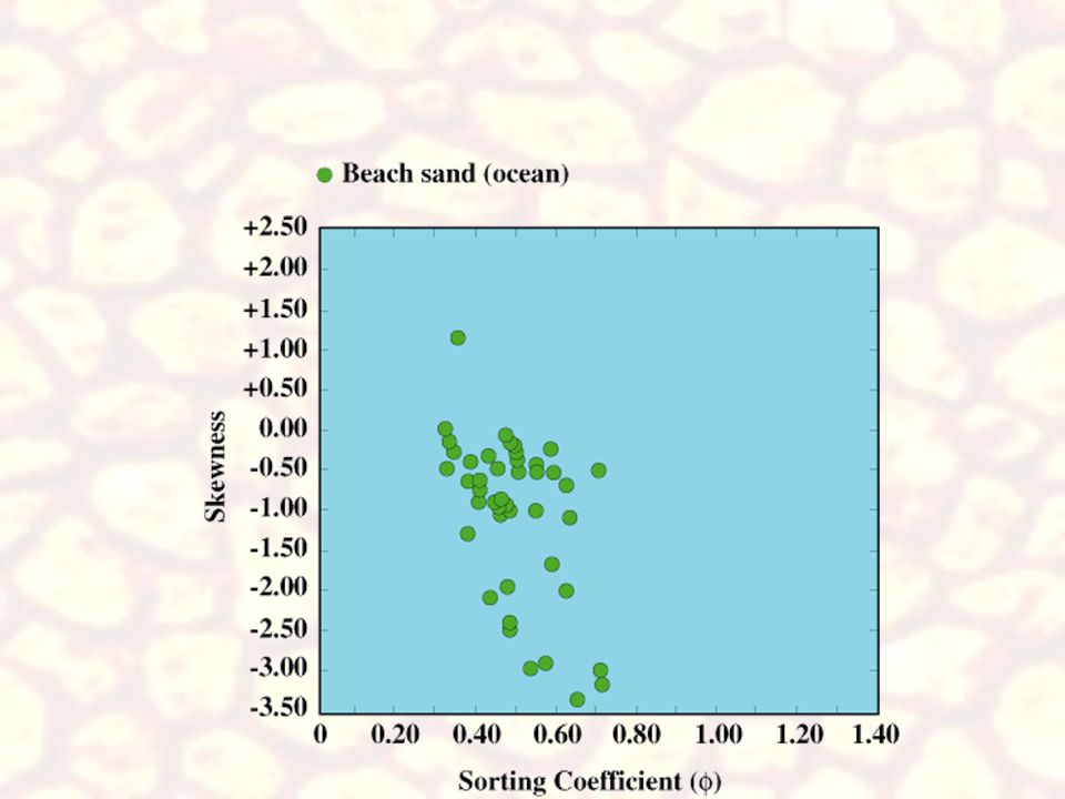
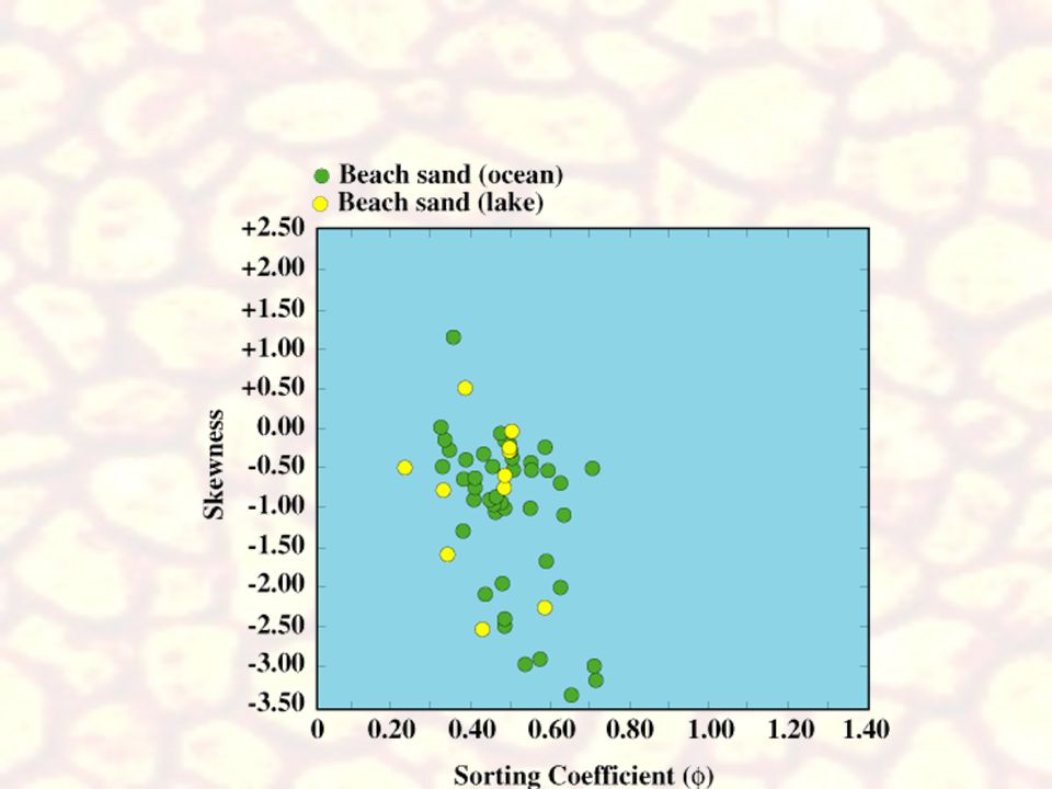


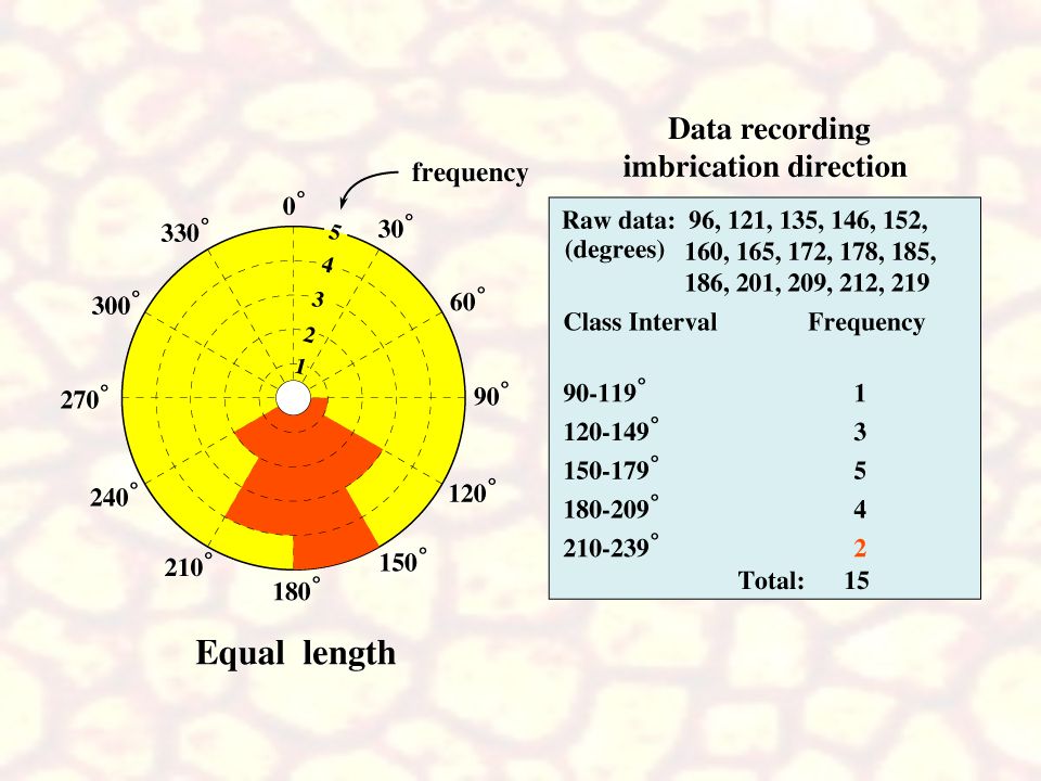


>")


 OCEAN/ESS 410 1.>")