1. Fundamental Concepts of Time and Frequency Metrology
Michael Lombardi
Chair, SIM Time and Frequency Metrology Working Group
National Institute of Standards and Technology (NIST)

2. NIST Laboratories in Boulder, Colorado, USA

3. There are three basic types of time and frequency information
Date and Time-of-Day
records when an event happened
Time Interval
duration between two events
Frequency
rate of a repetitive event

4. Two units of measurement in the International System (SI) apply to time and frequency metrology
Second (s)
standard unit for time interval
one of 7 base SI units
Hertz (Hz)
standard unit for frequency (s-1)
events per second
one of 21 SI units derived from base units

5. The units of time of day are defined as multiples of the SI second
1 minute = 60 second
1 hour = 60 minutes or 3600 seconds
1 day = 24 hours or 1440 minutes or seconds
1 year = days
Hour and minutes are based on the sexagesimal (base 60) system that is around 4000 years old. Days are based on the duodecimal (base 12) system that is at least 3500 years old.

6. The units of time interval are defined as fractional parts of the SI second
millisecond (ms), 10-3 s
microsecond (s), 10-6 s
nanosecond (ns), 10-9 s
picosecond (ps), s
femtosecond (fs), s
The sub-second units are all relatively new (within the last few hundred years) and all use the decimal (base 10) system.

7. The units of frequency are expressed in hertz, or in multiples of the hertz
hertz (Hz), 1 event or cycle per second
kilohertz (kHz), 103 Hz
megahertz (MHz), 106 Hz
gigahertz (GHz), 109 Hz

8. The relationship between frequency and time interval
We can measure frequency to get time interval, or we can measure time interval to get frequency. This is because frequency is the reciprocal of time interval:
Where T is the period of the signal in seconds f is the frequency in hertz
We can also express this as f = s-1 (the notation used to define the hertz in the SI).

9. Period
The period is the reciprocal of the frequency, expressed in units of time.

11. wavelength in meters = 300 / frequency in MHz
The wavelength is the length of one complete wave cycle, expressed in units of length.
wavelength in meters = 300 / frequency in MHz

12. Frequency Bands Higher frequencies means shorter wavelengths

13. “Everyday” frequencies in time and frequency metrology

14. Clocks and Oscillators

15. Clocks and Oscillators
A clock counts cycles of a frequency and records units of time interval, such as seconds, minutes, hours, and days. A clock consists of a frequency source, a counter, and a display. The frequency source is known as an oscillator.
A good example is a wristwatch. Most wristwatches contain an oscillator that generates cycles per second. After a watch counts cycles, it records that one second has elapsed.
A oscillator is a device that produces a periodic event that repeats at a nearly constant rate. This rate is called the resonance frequency. The best clocks contain the best oscillators.

16. The parts of a clock Repeating Motion + Counting Mechanism/Display
(from oscillator)
Earth Rotation
Pendulum Swing
Quartz Crystal Vibration
Cesium Atomic Vibration
Sundial
Clock Gears and Hands
Electronic Counter
Microwave Counter

17. What is a clock?
To most people, a clock is a device that displays the time of day. It answers perhaps the world’s most common question: What time is it now?
A frequency standard is some type of oscillator that defines the length of the second. It is reference or “time base” for the ticks of a clock.
However, metrologists often refer to clocks as either “time of day” measuring devices, or frequency standards, or both. You will probably hear the term “clock” used to mean both things in this meeting.

18. Synchronization and Syntonization
Synchronization is the process of setting two or more clocks to the same time.
Syntonization is the process of setting two or more oscillators to the same frequency.

19. Relationship of Frequency Accuracy to Time Accuracy

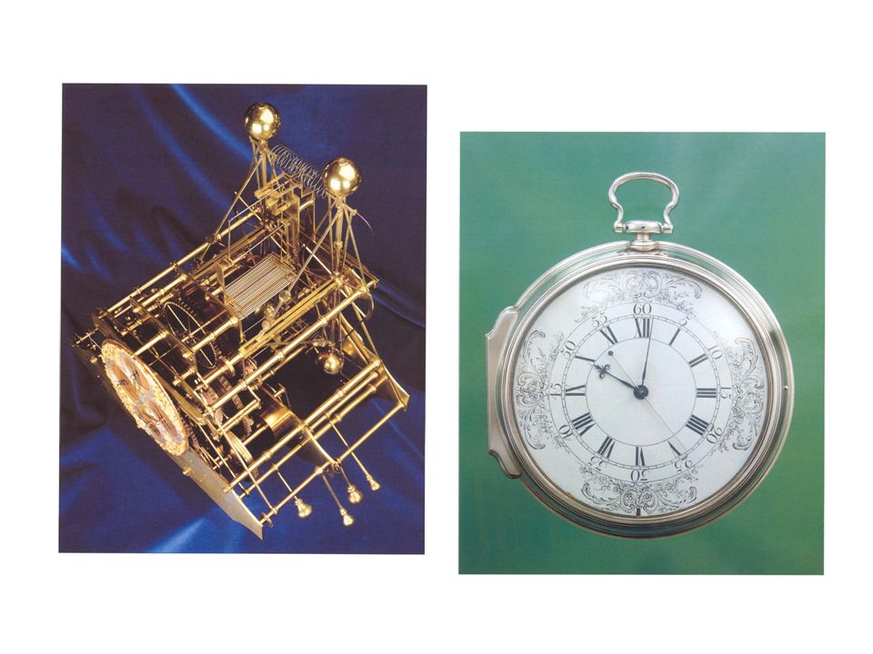
20. Clock performance – the “early” days

24. Clock performance in the modern era

25. Cesium Beam Primary Frequency Standards Designed at NBS/NIST

26. NIST-F1 Atomic Fountain Clock
Current accuracy (uncertainty):
3 x 10-16
26 trillionths of a second per day.
1 second in 105 million years.
The accuracy is equivalent to measuring distance from earth to sun (1.5 x 1011 m or 93 million miles) to uncertainty of about 45 µm (less than thickness of human hair).

27. NBS-1 NIST-F1 NIST-F2 Optical Standards
Improvements in Primary Frequency Standards: Optical Clocks
NBS-1
Frequency Uncertainty
NIST-F1
NIST-F2
Optical
Standards
Year

28. Clocks keep getting better and better!
Their performance has improved by about 13 orders of magnitude in the past 700 years, and by about 9 orders of magnitude (a factor of a billion) in the past 100 years. Further gains will occur when optical clocks are used as standards. Now, let’s take a quick look at the types of clocks that are found today in a time and frequency metrology lab

29. Quartz Oscillators
The most common type of oscillator – billions are manufactured every year! Quartz oscillators are mechanical oscillators that resonate based on the piezoelectric properties of synthetic quartz.
Excellent short term stability, but poor long term accuracy stability due to frequency drift and aging.
Highly sensitive to temperature and vibration.
A simple quartz oscillator (like those found in a stopwatch) is known as an XO. Test equipment usually contains either a TCXO (temperature controlled quartz oscillator), or an OCXO (oven controlled crystal oscillators). An OCXO offers the best performance.

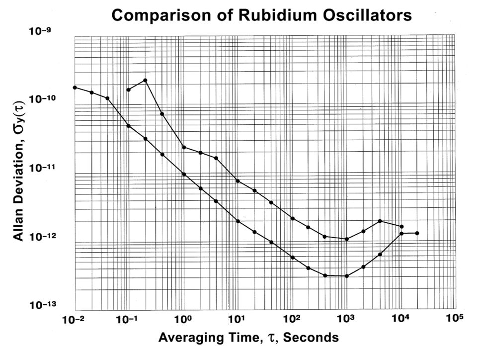
30. Rubidium Oscillators
The lowest priced atomic oscillators, used by many labs in the SIM Time Network.
A good laboratory standard. Their long-term accuracy and stability is much better than an OCXO, and they cost much less than a cesium oscillator.
Rubidium oscillators do not always have a guaranteed accuracy specification, but most are accurate to about 5  after a short warm up. However, their frequency often changes due to aging by parts in 1011 per month, so they require regular adjustments.

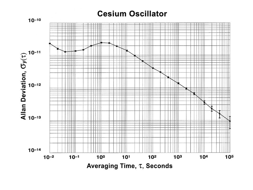
31. Cesium Oscillators
Cesium oscillators are the primary standard for time and frequency measurements and the basis for atomic time, because the second is defined with respect to energy transitions of the cesium atom.
Cesium oscillators are accurate to better than 1  after a short warm-up period, and have excellent long-term stability.
Cesium oscillators are expensive (usually $30,000 or more USD) to buy and maintain. The cesium beam tube is subject to depletion after a period of 5 to 10 years, and replacement costs are high.

32. GPS Disciplined Oscillators (GPSDO)

33. Oscillator Comparison (typical performance)
Parameter
/Device
Quartz OCXO
Rubidium
Cesium
GPSDO
Frequency accuracy after 30 minute warm-up
No guaranteed accuracy, must be set on frequency
5  10-10
1  10-12
Stability at 1 s
1  10-11
Parts in 1010
Stability at 1 day
1  10-10
2  10-12
1  10-13
2  10-13
Stability at 1 month
Parts in 109
5  10-11
Parts in 1014
Parts in 1015
Aging
1  / day
5  10-11/month
None, by definition
None, frequency is corrected by satellites
Cost (USD)
$200 to $2000
$1000 to $8000
$35000 to $75000
$1000 to $15000

34. Coordinated Universal Time (UTC)

35. What is a Time Scale?
An agreed upon system for keeping time, based on a common definition of the second. Seconds are then counted to form longer time intervals like minutes, hours, days, and years.
Time scales serve as a reference for time-of-day, time interval, and frequency.

36. How is the SI second defined?
Pendulums or quartz oscillators were once used as national standards at NIST and elsewhere, but they were never used to define the second. The definition of the second went directly from astronomical to atomic time.
Before 1956, the second was defined based on the length of the mean solar day and was called the mean solar second.
From 1956 to 1967, the second was defined based on a fraction of the tropical year and was called the ephemeris second.
Since 1967, the second has been defined based on oscillations of the cesium atom and is called the atomic second, or cesium second.

37. SI Definition of the Second
The duration of 9,192,631,770 periods of the radiation corresponding to the transition between two hyperfine levels of the ground state of the cesium-133 atom.
=> Defined by Markowitz/Hall (USNO) & Essen/Parry (NPL), 1958.
=> Ratified by the SI in 1967.

38. Coordinated Universal Time (UTC)
UTC is an atomic time scale based on the SI definition of the second.
UTC is computed by the International Bureau of Weights and Measures (BIPM) in France. They collect data from about 400 atomic oscillators located at more than 60 laboratories.
Six SIM labs currently contribute to UTC:
CENAM, CENAMEP, INTI, NIST, NRC, ONRJ
UTC is a virtual time scale, computed by the BIPM after the data is collected. Therefore, no lab can distribute or broadcast UTC.
Many laboratories maintain local, real-time versions of UTC that they distribute as a measurement reference. Most of the real-time versions of UTC are within 100 nanoseconds of the official UTC time scale.

39. UTC is the Official Reference for Time-Of-Day
Clocks synchronized to UTC display the same second (and normally the same minute) all over the world. However, since UTC is used internationally, it ignores local conventions like time zones and daylight saving time (DST). The UTC hour refers to the hour at the Prime Meridian which passes through Greenwich, England.

40. UTC is the Official Reference for Time Interval
Time interval is the duration between two events measured in seconds or sub-seconds (milliseconds, microseconds, nanoseconds, picoseconds).
All time interval measurements are referenced to the best realization of the SI second as computed by the BIPM when they derive UTC.
Clocks can be synchronized to UTC by using an On-Time Marker (OTM) that coincides as closely as possible with the arrival of the Coordinated Universal Time (UTC) second. Systems such as GPS can provide this OTM.

41. UTC is the Official Reference for Frequency
UTC runs at an extremely stable rate with an uncertainty measured in parts in 1015 or less. Therefore, it serves as the international reference for all frequency measurements.

42. Measuring Frequency Accuracy

43. Four Parts of a Calibration
Device Under Test (DUT)
Can be a tuning fork or a stopwatch or timer
Can be a quartz, rubidium, or cesium oscillator
Traceable Reference
Can be any reference that can be linked back to the SI
Calibration Method
The measurement system and procedure used to collect data
Calibration Result
The result must be accompanied by an uncertainty analysis

44. Calibration
Comparison between a reference and a device under test (DUT) that is conducted by collecting measurement data. Calibration results should include a statement of measurement uncertainty, and should establish a traceability chain back to the International System of Units (SI).

45. Test Uncertainty Ratio (TUR)
Common sense tells us that the reference must have a smaller uncertainty than the device under test. The performance ratio between the reference and the device under test is called the test uncertainty ratio.
ISO Guide requires a complete uncertainty analysis. However, if a 10:1 TUR is maintained, the uncertainty analysis becomes much easier because you don’t have to worry as much about the uncertainty of the reference.

46. For this DUT
Use this reference
Quartz
Rubidium
Cesium
GPSDO
National Standard
GPSDO, allow at least 1 week, maybe longer, for the calibration
Normally not calibrated unless a national standard is used.

47. Frequency Accuracy (Offset)
The degree of conformity of a measured value to its definition at a given point in time. Accuracy tells us how closely an oscillator produces its nominal or nameplate frequency.

48. What else is it called? Frequency Offset Frequency Error
Frequency Bias
Frequency Difference
Relative Frequency
Fractional Frequency
Accuracy

49. Resolution
The smallest unit that a measurement can determine. For example, if a 10-digit frequency counter is used to measure a 10 MHz signal, the resolution is .001 Hz, or 1 mHz.
== 10-digit counter
The “single shot” resolution is determined by the quality of the measurement system, but more resolution can usually be obtained by averaging.

50. Using a Frequency Counter

51. Estimating Frequency Offset (accuracy) in the Frequency Domain (a measurement made with respect to frequency)
fmeasured is the reading from an instrument, such as a frequency counter
fnominal is the frequency labeled on the oscillator’s output

52. Phase
Time and frequency metrologists usually use units of time to talk about phase, rather than using units of phase angle. Therefore “time plot”, “time difference plot”, and “phase plot” usually mean the same thing.
The time interval for a 1° phase change is inversely proportional to the frequency. If the frequency of a signal is given by f, then the time tdeg (in seconds) corresponding to 1° of phase is:
tdeg = 1 / (360f) = T / 360
Therefore, a 90° phase shift on a 1 MHz signal corresponds to a time shift of about 250 nanoseconds. This same answer can be obtained by taking the period of 1 MHz (1000 nanoseconds) and dividing by 4.

53. Phase Comparisons
A common method used to estimate frequency accuracy in the time domain.
Phase comparisons measure the change in phase (or phase deviation) of the DUT signal relative to the reference during a calibration. When expressed in time units, this quantity is sometimes called t , spoken as “delta-t”, which simply means the change in time.

54. Using an Oscilloscope

55. Phase Comparison
The frequency of the device under test can be measured by comparing the phase of its signal to the signal from the reference. t1 t2 t3 f1
Reference f2
Device Under Test
t`1
t`2
t`3

56. Phase Difference, t or Φ
Signal 1
Signal 1
Signal 2
Reference frequency
Signal 2
Time Interval Counter
Device under test

57. Accumulated Phase Difference
Signal 1
Signal 2

58. Frequency accuracy is computed from the slope of the phase

59. Using a Time Interval Counter

60. Estimating Frequency Offset (accuracy) in the Time Domain (a measurement made with respect to time)
The quantity t is the phase change expressed in time units, estimated by the difference of two readings from a time interval counter or oscilloscope. T is the duration of the measurement, also expressed in time units.

61. Frequency Domain and Time Domain
You might find it confusing that time measurements made with a time interval counter can be made to estimate frequency uncertainty, or that a frequency measurement can be used to estimate time interval uncertainty.
The word “domain” just means that the equations we use to analyze the measurement are made with respect to either frequency or time units. For example, in a frequency domain measurement, the mathematical analysis is done with respect to frequency. In a time domain measurement, the mathematical analysis is done with respect to time.

62. Frequency Domain
In the frequency domain, voltage and power are measured as functions of frequency. For example, a spectrum analyzer separates signals into their frequency components and displays the power level at each frequency. An ideal sine wave (perfect frequency) appears as a spectral line of zero bandwidth in the frequency domain. Real sine wave outputs are always noisy, so the spectral lines always have a finite bandwidth.

63. Time Domain
In the time domain, voltage and power are measured as functions of time. Instruments such as time interval counters and oscilloscopes are used to measure signals in the time domain. These signals are generally sine or square waves. An ideal sine wave (perfect frequency) would not produce any noise. For example, an ideal 5 MHz sine wave would not generate a signal at any frequency other than 5 MHz. The period of the sine wave would always be exactly 200 ns, its bandwidth would be zero, and its frequency uncertainty would also be zero. Obviously, no such signals exist in the real world.

64. Two important things to remember
Frequency accuracy is normally expressed as a dimensionless number (unitless). You can convert the offset to units of frequency by multiplying the nominal frequency by the offset. For example, a 10 MHz oscillator with a frequency offset of 1 x has a offset of Hz.
(1 x 107) (1 x 10-11) = 1 x 10-4 = Hz
We get the same answer in the frequency domain or the time domain:

65. Measuring Frequency Stability

66. Stability
Stability indicates how well an oscillator can produce the same time and frequency offset over a given period of time. Stability doesn’t indicate whether the time or frequency is “right” or “wrong”, but only whether it stays the same.
In contrast, accuracy indicates how well an oscillator has been set on time or set on frequency.

67. The relationship between accuracy and stability

68. Estimating Stability
Stability is estimated with statistics that evaluate the frequency fluctuations of an oscillator that occur over time. The most common statistic used to estimate frequency stability is the Allan deviation.
Short-term stability usually refers to intervals of less than 100 seconds.
Long-term stability can refer to any interval greater than 100 seconds, but usually refers to periods of 1 day or longer.

69. Why standard deviation doesn’t work with oscillators
Consider this graph of the growth of a child who was 20 inches tall at birth, and 67 inches tall at age 16.
At age 8, the child’s average height was about 36 inches, and the estandard dviation was about 8 inches. By age 16, the average height had increased to 46 inches, and the standard deviation was about 14 inches.
These numbers are meaningless! Taking the mean and the standard deviation from the mean is pointless if the data has a trend, or is “non-stationary”. That’s why standard deviation is seldom used in time and frequency.

70. What is the Allan Deviation (ADEV)?
It’s a statistic used to estimate frequency stability. It was named after Dave Allan, a physicist who retired from NIST in He first published the statistic in 1966.
The mathematical notation is σy(τ). The y means frequency and the τ refers to the averaging time. The σ is the same notation we use for standard deviation, and ADEV refers to the deviation of the frequency over a given averaging time.
ADEV is computed by taking the differences between successive pairs of data points. This differencing removes the trend or slope contributed by the frequency offset. This is necessary because data with a trend is non-stationary, and never converges to a particular mean. By removing the trend, we can make the data converge to a mean.
Because the slope contributed by the frequency offset is gone, ADEV is only useful for computing stability, and not accuracy. Keep in mind that ADEV has EVERYTHING to do with stability, and NOTHING to do with accuracy.

71. Using the Allan Deviation with time domain data
where:
xi is a set of equally spaced phase measurements in time units, such as data from a time interval counter
N is the number of values in the xi series
 (tau) is the measurement or sampling interval
m is the averaging factor
ADEV is computed using an iterative method (multiple passes through a loop). Normally, ADEV is computed using the octave method, so m is doubled on each pass. For example, stability would be estimated at 1, 2, 4, 8, 16, 32 s, etc. But it is possible to increment m by 1 each time, and calculate stability for every possible averaging time. That takes longer, but reveals more information.

72. Using time interval measurements to estimate stability

73. Using time measurements to estimate stability (cont.)
2.2 x is the sum of the first differences squared
1 second data is combined to estimate stability over longer periods

74. Noise Floor
Allan deviation graphs show stability estimates at different averaging times. These estimates improve until the devices reaches its noise floor. The noise floor is the point where more averaging doesn’t help; you’ll get the same answer or a worse answer if you continue to average.
Oscillator specification sheets usually only provide stability estimates out to the point where the noise floor is reached. For example, if an oscillator’s specification sheet only shows stability estimates out to an average time of 10 seconds, you’ll know that the stability at longer intervals (like 1 hour or 1 day) is worse than the stability at 10 seconds.

75. How long does it take for a oscillator to reach its noise floor?
Quartz
< 10 s, sometimes < 1 s
Rubidium
1000 s
Cesium
Several days to 30 days
GPSDO
The noise continuously averages down, because the GPS frequency is being always being steered and corrected to agree with UTC, which is the best approximation of the SI second

79. A few things to remember about stability
It is important to never confuse accuracy with stability. This is a mistake that is commonly made by people when they talk about clocks.
The accuracy over a given averaging time can never be better than the stability over that same averaging time. In most cases, the stability will be a smaller, more impressive number than the accuracy.