1. General Concepts of Time and Frequency Metrology
Michael Lombardi

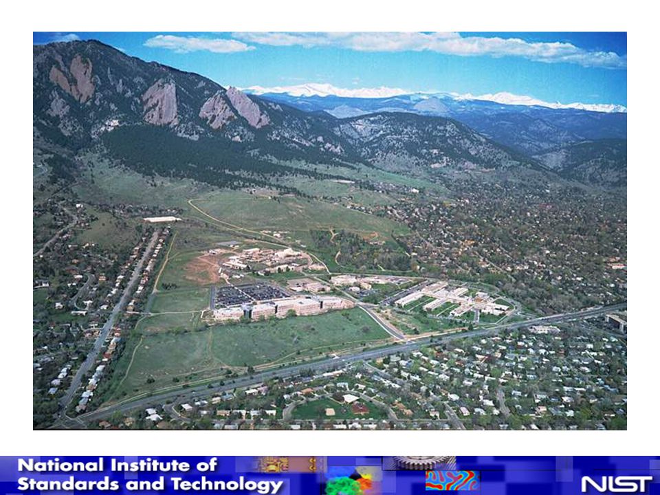
2. NIST Boulder Laboratories

4. Types of Time and Frequency Information
Date and Time-of-Day
records when an event happened
Time Interval
duration between two events
Frequency
rate of a repetitive event

5. Two units of measurement in the International System (SI) apply to time and frequency metrology
Second (s)
standard unit for time interval
one of 7 base SI units
Hertz (Hz)
standard unit for frequency (s-1)
events per second
one of 21 SI units derived from base units

6. The relationship between frequency and time
We can measure frequency to get time interval, and vice versa, because the relationship between frequency and time interval is known. Frequency is the reciprocal of time interval:
Where T is the period of the signal in seconds, and f is the frequency in hertz. We can also express this as f = s-1 (the notation used to define the hertz in the SI).

7. Period
The period is the reciprocal of the frequency, and vice versa. Period is expressed in units of time.

8. An Oscillating Sine Wave

9. Units of Time Interval second (s) millisecond (ms), 10-3 s
microsecond (s), 10-6 s
nanosecond (ns), 10-9 s
picosecond (ps), s
femtosecond (fs), s

10. Units of Frequency hertz (Hz), 1 event per second
kilohertz (kHz), 103 Hz
megahertz (MHz), 106 Hz
gigahertz (GHz), 109 Hz

11. An Oscillating Sine Wave

12. wavelength in meters = 300 / frequency in MHz
The wavelength is the length of one complete wave cycle. Wavelength is expressed in units of length.
wavelength in meters = 300 / frequency in MHz

13. Frequency Bands Higher frequencies means shorter wavelengths

14. We Use a Wide Range of Frequencies “Everyday” frequencies in time and frequency metrology

15. Clocks and Oscillators

16. Clocks and Oscillators
A clock is a device that counts cycles of a frequency and records units of time interval, such as seconds, minutes, hours, and days. A clock consists of a frequency source, a counter, and a output device. The frequency source is known as an oscillator.
A good example is a wristwatch. Most wristwatches contain an oscillator that generates cycles per second. After a watch counts cycles, it can record that one second has elapsed.
A oscillator is a device that produces a periodic event that repeats at a nearly constant rate. This rate is called the resonance frequency. Since the best clocks contain the best oscillators, the evolution of timekeeping has been a continual quest to find better and better oscillators.

17. Synchronization & Syntonization
Synchronization is the process of setting two or more clocks to the same time.
Syntonization is the process of setting two or more oscillators to the same frequency.

18. Relationship of Frequency Accuracy to Time Accuracy

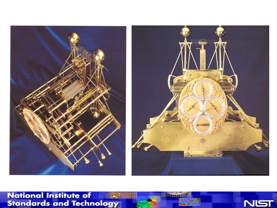
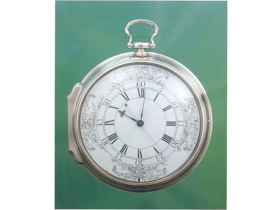
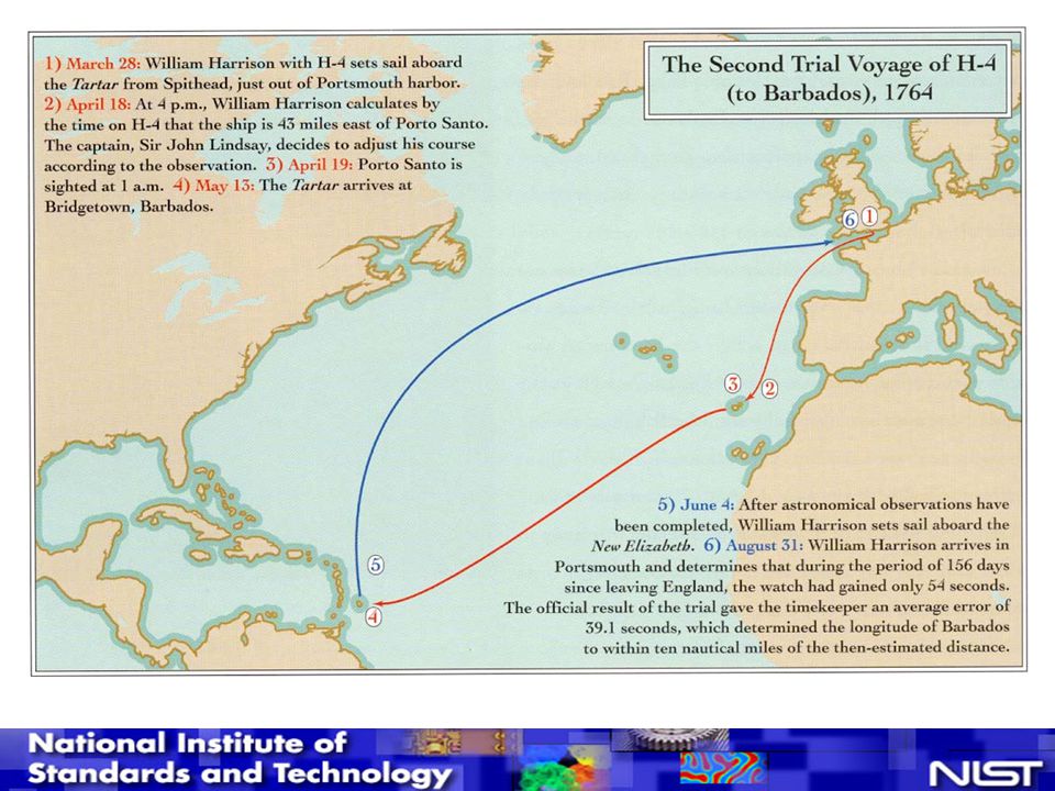
19. The Evolution of Time and Frequency Standards - Part I

24. The Evolution of Time and Frequency Standards - Part II

25. Clocks and oscillators keep getting better and better
The performance of time and frequency standards has improved by about 13 orders of magnitude in the past 700 years, and by about 9 orders of magnitude (a factor of a billion) in the past 100 years.

26. Quartz Oscillators
Mechanical oscillators that resonate based on the piezoelectric properties of synthetic quartz.
Excellent short term stability, but poor long term accuracy stability due to frequency drift and aging.
Highly sensitive to environmental parameters such as temperature and vibration.
A simple quartz oscillator (like those is a stopwatch) is known as an XO. Test equipment usually contains either a TCXO (temperature controlled quartz oscillator), or an OCXO (oven controlled crystal oscillators). An OCXO offers the best performance.

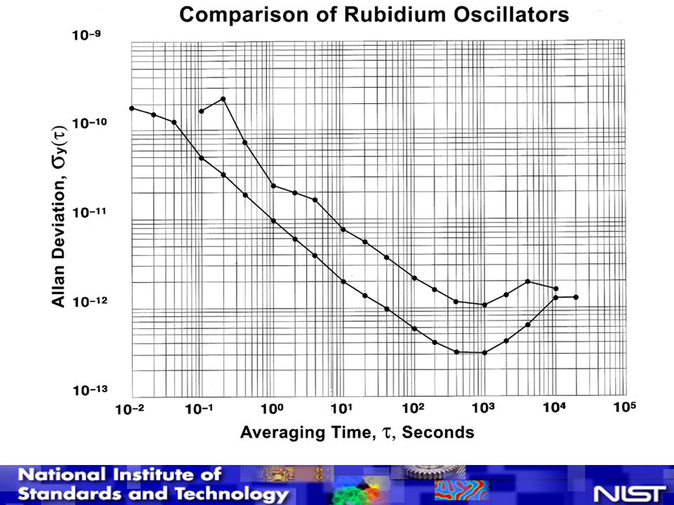
27. Rubidium Oscillators The lowest priced atomic oscillator.
A good laboratory standard. Their long-term accuracy and stability is much better than an OCXO, and they cost much less than a cesium oscillator.
Rubidium oscillators do not always have a guaranteed accuracy specification, but most are accurate to about 5  after a short warm up. However, their frequency often changes due to aging by parts in 1011 per month, so they will require periodic adjustment to get the best possible accuracy.

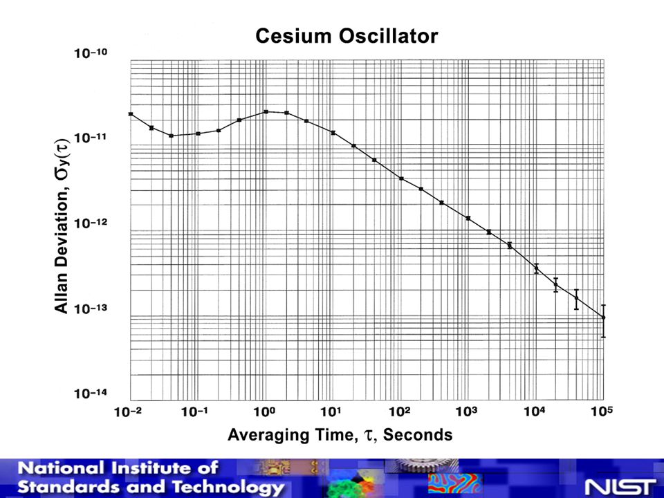
28. Cesium Oscillators
Cesium oscillators are the primary standard for time and frequency measurements and the basis for atomic time, because the second is defined with respect to energy transitions of the cesium atom.
Cesium oscillators are accurate to better than 1  after a short warm-up period, and have excellent long-term stability.
However, cesium oscillators are expensive (usually $30,000 or more USD), and have relatively high maintenance cost. The cesium beam tube is subject to depletion after a period of 5 to 10 years, and replacement costs are high.

29. GPS Disciplined Oscillators (GPSDO)

30. Oscillator Comparison (typical performance)
Parameter
/Device
Quartz OCXO
Rubidium
Cesium
GPSDO
Frequency accuracy after 30 minute warm-up
No guaranteed accuracy, must be set on frequency
5  10-10
1  10-12
Stability at 1 s
1  10-11
Parts in 1010
Stability at 1 day
1  10-10
2  10-12
1  10-13
2  10-13
Stability at 1 month
Parts in 109
5  10-11
Parts in 1014
Parts in 1015
Aging
1  / day
5  10-11/month
None, by definition
None, frequency is corrected by satellites
Cost (USD)
$200 to $2000
$1000 to $8000
$25000 to $50000
$2000 to $15000

31. Coordinated Universal Time (UTC)

32. What is a Time Scale?
An agreed upon system for keeping time, based on a common definition of the second. Seconds are then counted to form longer time intervals like minutes, hours, days, and years.
Time scales serve as a reference for time-of-day, time interval, and frequency.

33. How is the SI second defined?
Pendulums or quartz oscillators were never used to define the second. We went directly from astronomical to atomic time.
Before 1956, the second was defined based on the length of the mean solar day. Called the mean solar second.
From 1956 to 1967, the second was defined based on a fraction of the tropical year. Called the ephemeris second.
Since 1967, the second has been defined based on oscillations of the cesium atom. Called the atomic second, or cesium second.
The change to the cesium second in 1967 officially began the era of atomic timekeeping. Prior to 1967, time was kept by astronomical observations.

34. SI Definition of the Second
The duration of 9,192,631,770 periods of the radiation corresponding to the transition between two hyperfine levels of the ground state of the cesium-133 atom.
=> Defined by Markowitz/Hall (USNO) & Essen/Parry (NPL), 1958.
=> Ratified by the SI in 1967.

35. Coordinated Universal Time (UTC)
UTC is an internationally recognized atomic time scale based on the SI definition of the second.
The average value of UTC is computed by the International Bureau of Weights and Measures (BIPM) in France. They collect data from over 250 atomic oscillators located at nearly 60 national metrology institutes.
UTC is a paper time scale, computed by the BIPM after the data is collected. Therefore, no one can distribute or broadcast the “real” UTC.
Fortunately, national labs like NIST, CENAM, NRC, CENAMEP, and ONRJ maintain real-time versions of UTC that they do distribute and broadcast as a measurement reference. Most of the real-time versions of UTC are usually within 100 nanoseconds of the post processed UTC time scale.

36. UTC is the Official Reference for Time-Of-Day
Clocks synchronized to UTC display the same second (and normally the same minute) all over the world. However, since UTC is used internationally, it ignores local conventions like time zones and daylight saving time (DST). The UTC hour refers to the hour at the Prime Meridian which passes through Greenwich, England. California time, for example, will differ from UTC by either 7 or 8 hours, depending upon whether or not DST is in effect.

37. UTC is the Official Reference for Time Interval
Time interval is the duration between two events. In time and frequency metrology, it is normally expressed in seconds or sub-seconds (milliseconds, microseconds, nanoseconds, picoseconds).
Since UTC is based on the SI definition of the second, all time interval measurements are referenced to its one second pulses. By counting the pulses, time is kept.
Timing systems are synchronized to UTC by using an On-Time Marker (OTM), consisting of a pulse or signal that coincides as closely as possible with the arrival of the Coordinated Universal Time (UTC) second. The uncertainty of the OTM indicates the time interval between its arrival and the UTC second

38. UTC is the Official Reference for Frequency
UTC runs at an extremely stable rate with an uncertainty measured in parts in Therefore, it serves as the international reference for all frequency measurements

39. Units of measurements kg m s A K cd mol SI Base Units SI Derived Units
Electric
Current
ampere
Mass
kilogram
Length
meter
Time
second
Temperature
kelvin
Luminous
Intensity
candela
Amount of
Substance
mole kg m s A K cd
mol S
Coordinated Time
international atomic time
TAI K
Celsius
Temperature
0Celsius 0C
cd sr
Luminous Flux
lumen lm
SI Derived Units
s-1
Frequency
hertz Hz
kg m s-2
Force
newton N
m-2cd sr
Illuminance
lux lx
kg m2s-2
Energy
joule J
kg m-1s-2
Pressure
pascal Pa
S A
Electric charge
coulomb C
kg m s-3
Power
watt W
kg m2s-3 A-1
Electric Potential
volt V
kg m2s-3A-2
Resistance
ohm 
Non-SI units
recognized
for use with SI
day: 1 d = s
hour: 1 h = 3600 s
minute: 1 min = 60 s
liter: 1 l = 10-3 m3
ton: 1 t = 103 kg
degree: 10 = (/180) rad
minute: 1’ = (/10800)rad
second: 1” = (/648000)rad
electronvolt: 1 eV  x J
unified atomic mass unit: 1 u  x kg
sr: the steradian is the supplementary
SI unit of solid angle (dimensionless)
Time interval (frequency) is the quantity that can be determined with the highest accuracy. It can be measured with an accuracy greater than 1 part in With the help of satellites, it is possible to compare the time scales kept by the national laboratories, worldwide, to an accuracy of ~1 ns. Time, therefore, plays a central role in metrology and in the definitions of SI units.
The SI consists of seven base units and a number of derived units, as shown above. Shown on the next page are the units that do NOT depend on the unit of time.
R. J. Douglas, et. al, "Frequency Standards, Timekeeping, and Traceable Services at the National Research Council of Canada," Proc. 28th Ann. Precise Time & Time Interval (PTTI) Applications & Planning Meeting, pp , 1996.
The chart above, and the one on the next page, were provided by R.J. Douglas, National Research Council Canada, 1997.
E. R. Cohen & B. N. Taylor, “The Fundamental Physical Constants,” Physics Today, pp. BG7-BG14, August 1997.
s-1
Activity
becquerel Bq
rad: the radian is the supplementary
SI unit of plane angle (dimensionless)
kg-1 m2s4 A2
Capacitance
farad F
kg m2s-2A-1
Magnetic Flux
weber Wb
m2s-1
Absorbed Dose
gray Gy
kg-1 m2s3 A2
Conductance
siemens S
kg m2s-2A-2
Inductance
henry H
m2s-2
Dose Equivalent
sievert Sv
kg s-2 A-1
Conductance
siemens S
Electromagnetic
measurement units
Health related
measurement units

40. Time is the ultimate measurement!
If the kilogram is replaced by a Watt balance, mass would be ultimately defined by the second, like the meter and other units.
This would leave only the Kelvin and the amount of substance as base units that do not depend on the second.
The second can be measured with more resolution and less uncertainty than any other quantity. NIST can measure the second with an uncertainty of about 4 x

41. Where the SI second is not needed
SI Base Units
Mass
kilogram
Temperature
kelvin
Amount of
Substance
mole kg K
mol K
Celsius
Temperature
0Celsius 0C
SI Derived Units
sr: the steradian is the supplementary
SI unit of solid angle (dimensionless)
Time interval (frequency) is the quantity that can be determined with the highest accuracy. It can be measured with an accuracy greater than 1 part in With the help of satellites, it is possible to compare the time scales kept by the national laboratories, worldwide, to an accuracy of ~1 ns. Time, therefore, plays a central role in metrology and in the definitions of SI units.
The SI consists of seven base units and a number of derived units, as shown above. Shown on the next page are the units that do NOT depend on the unit of time.
R. J. Douglas, et. al, "Frequency Standards, Timekeeping, and Traceable Services at the National Research Council of Canada," Proc. 28th Ann. Precise Time & Time Interval (PTTI) Applications & Planning Meeting, pp , 1996.
The chart above, and the one on the next page, were provided by R.J. Douglas, National Research Council Canada, 1997.
E. R. Cohen & B. N. Taylor, “The Fundamental Physical Constants,” Physics Today, pp. BG7-BG14, August 1997.
Non-SI units
recognized
for use with SI
ton: 1 t = 103 kg
degree: 10 = (/180) rad
minute: 1’ = (/10800)rad
second: 1” = (/648000)rad
unified atomic mass unit: 1 u  x kg
rad: the radian is the supplementary
SI unit of plane angle (dimensionless)

42. Where the SI second is not needed
SI Base Units
Temperature
kelvin
Amount of
Substance
mole K
mol K
Celsius
Temperature
0Celsius 0C
SI Derived Units
sr: the steradian is the supplementary
SI unit of solid angle (dimensionless)
Time interval (frequency) is the quantity that can be determined with the highest accuracy. It can be measured with an accuracy greater than 1 part in With the help of satellites, it is possible to compare the time scales kept by the national laboratories, worldwide, to an accuracy of ~1 ns. Time, therefore, plays a central role in metrology and in the definitions of SI units.
The SI consists of seven base units and a number of derived units, as shown above. Shown on the next page are the units that do NOT depend on the unit of time.
R. J. Douglas, et. al, "Frequency Standards, Timekeeping, and Traceable Services at the National Research Council of Canada," Proc. 28th Ann. Precise Time & Time Interval (PTTI) Applications & Planning Meeting, pp , 1996.
The chart above, and the one on the next page, were provided by R.J. Douglas, National Research Council Canada, 1997.
E. R. Cohen & B. N. Taylor, “The Fundamental Physical Constants,” Physics Today, pp. BG7-BG14, August 1997.
Non-SI units
recognized
for use with SI
ton: 1 t = 103 kg
degree: 10 = (/180) rad
minute: 1’ = (/10800)rad
second: 1” = (/648000)rad
unified atomic mass unit: 1 u  x kg
rad: the radian is the supplementary
SI unit of plane angle (dimensionless)

43. Atomic Time Scales
TAI and UTC are both atomic time scales based on the cesium definition of the second.
International Atomic Time (TAI)
TAI runs at the same frequency as UTC (this frequency is determined by the BIPM), but is not corrected for leap seconds. TAI is seldom used by the general public. It is an “internal” time scale used by the BIPM and national laboratories like NIST.
Coordinated Universal Time (UTC)
UTC is TAI corrected for leap seconds so that it stays within 0.9 seconds of UT1.

44. Leap Seconds
An integer second added to atomic time (UTC) to keep it within 0.9 seconds of the most widely used astronomical time scale (UT1).
Leap seconds usually occur on June 30th or December 31st.
On average, about 7 are needed every 10 years, suggesting that the long term frequency offset of the Earth is about 2 x However, the Earth both speeds up and slows down, making the occurrence of leap seconds cyclical. No leap seconds were needed in 1999 to 2004, but there was a leap second on December 31, 2005.
The biggest reason that so many leap seconds have been needed is that the atomic second (cesium) was defined relative to the ephemeris second (which served as the SI second in 1958), and not the mean solar second.

45. Implementation of Leap Seconds
When a leap second occurs, one minute has 61 seconds. This effectively stops UTC for one second so that UT1 can catch up. The sequence is:
23 hours, 59 minutes, 59 seconds
23 hours, 59 minutes, 60 seconds
0 hours, 0 minutes, 0 seconds

46. The place of time in metrology
The SI second is central to metrology.
It is a truly independent unit which is defined in term of physics without the need for another unit.
It is the basis for most other units.
Unlike mass, it does not depend on the history of an artifact (Sèvres Grand K is measured once every 40 years or so).
The Silicon balls are just that after all…

47. Uncertainties of physical realizations of the base SI units

48. Time and Frequency Measurement Basics

49. Four Parts of a Calibration
Device Under Test (DUT)
Can be a tuning fork or a stopwatch or timer
Can be a quartz, rubidium, or cesium oscillator
Traceable References
(transfer standards like WWV, WWVB, LORAN, GPS, or any reference that provides a link back to the SI)
Calibration Method
(measurement system and procedure used to collect data)
Uncertainty Analysis
(statistics and data reduction)

50. Calibration
Comparison between a reference and a device under test (DUT) that is conducted by collecting measurement data. Calibration results should include a statement of measurement uncertainty, and should establish a traceability chain back to the International System of Units (SI).

51. Test Uncertainty Ratio (TUR)
Performance ratio between the Reference and the device under test.
United States Mil Spec 45662A (now obsolete) required a 4:1 TUR.
ISO Guide requires a complete uncertainty analysis. However, if a 10:1 TUR is maintained, the uncertainty analysis becomes much easier, since you don’t have to worry as much about the uncertainty of the reference (it is “lost in the noise”).

52. For this DUT
Use this reference
TXCO
OCXO
Rubidium
Cesium
GPSDO
GPSDO, allow at least 1 week, maybe longer, for the calibration
Normally accepted as self-calibrating standard using manufacturer’s specifications. For an absolute delay calibration, send to NIST or another NMI.

53. Frequency Accuracy (Offset)
The degree of conformity of a measured value to its definition at a given point in time. Accuracy tells us how closely an oscillator produces its nominal or nameplate frequency.
What we use for definition of accuracy. Nameplate frequency is what frequency should be at, say 5 MHz.

54. What else is it called? Frequency Offset Frequency Error
Frequency Bias
Frequency Difference
Relative Frequency
Fractional Frequency
Accuracy

55. Resolution
The smallest unit that a measurement can determine. For example, if a 10-digit frequency counter is used to measure a 10 MHz signal, the resolution is .001 Hz, or 1 mHz.
== 10-digit counter
The “single shot” resolution is determined by the quality of the measurement system, but more resolution can usually be obtained by averaging.

56. Using a Frequency Counter

57. Estimating Frequency Offset (accuracy) in the Frequency Domain (a measurement made with respect to frequency)
fmeasured is the reading from an instrument, such as a frequency counter
fnominal is the frequency labeled on the oscillator’s output

58. Phase
The position of a point in time (instant) on a waveform cycle. One cycle constitutes 360° of phase. One radian of phase equals approximately 57.3°.
In time and frequency metrology, the phase difference is usually stated in units of time, rather than in units of phase angle. What we often call a phase plot might properly be known as a time plot, or a time difference plot, but the concept is the same. The time interval for 1° of phase is inversely proportional to the frequency. If the frequency of a signal is given by f, then the time tdeg (in seconds) corresponding to 1° of phase is:
tdeg = 1 / (360f) = T / 360
Therefore, a 45° phase shift on a 60 kHz signal corresponds to a time shift of about 2.1 microseconds. This same answer can be obtained by taking the period of 60 kHz (16.67 microseconds) and dividing by 8.

60. Phase Comparisons
Used to estimate frequency offset in the time domain.
Phase comparisons measure the change in phase (or phase deviation) of the DUT signal relative to the reference during a calibration. When expressed in time units, this quantity is sometimes called t , spoken as “delta-t”, which simply means the change in time.

61. Using an Oscilloscope

62. Phase Comparison
The frequency of the device under test can be measured by comparing the phase of its signal to the signal from the reference. t1 t2 t3 f1
Reference f2
Device Under Test
t`1
t`2
t`3

63. Phase Difference, t or Φ
Signal 1
Signal 1
Signal 2
Reference frequency
Signal 2
Time Interval Counter
Device under test

64. Accumulated Phase Difference
Signal 1
Signal 2

65. A Sample Phase Plot

66. Using a Time Interval Counter

67. Estimating Frequency Offset (accuracy) in the Time Domain (a measurement made with respect to time)
The quantity t is the phase change expressed in time units, estimated by the difference of two readings from a time interval counter or oscilloscope
T is the duration of the measurement, also expressed in time units

68. Frequency Domain versus Time Domain
You might find it confusing that time measurements made with a time interval counter can be made to estimate frequency uncertainty, or that a frequency measurement can be used to estimate time interval uncertainty.
Some measurements are made in the frequency domain and some are made in the time domain. The word “domain” just means that the equations we use to analyze the measurement are made with respect to either frequency or time units. For example, in a frequency domain measurement, the mathematical analysis is done with respect to frequency. In a time domain measurement, the mathematical analysis is done with respect to time.

69. Frequency Domain
In the frequency domain, voltage and power are measured as functions of frequency. A spectrum analyzer is one instrument that can analyze signals in the frequency domain. It does so by separating signals into their frequency components and displaying the power level at each frequency. An ideal sine wave (perfect frequency) appears as a spectral line of zero bandwidth in the frequency domain. Real sine wave outputs are always noisy, so the spectral lines have a finite bandwidth, as shown in the graphic.

70. Time Domain
In the time domain, voltage and power are measured as functions of time. Instruments such as time interval counters and oscilloscopes are used to measure signals in the time domain. These signals are generally sine or square waves. An ideal sine wave (perfect frequency) would not produce any noise. For example, an ideal 5 MHz sine wave would not generate a signal at any frequency other than 5 MHz. The period of the sine wave would always be exactly 200 ns, its bandwidth would be zero, and its frequency uncertainty would also be zero. Obviously, such signals do not exist in the real world.

71. Two important things to remember
Frequency accuracy is normally expressed as a dimensionless number. You can convert the offset to units of frequency by multiplying the nominal frequency by the offset. For example, a 10 MHz oscillator with a frequency offset of 1 x has a offset of Hz.
(1 x 107) (1 x 10-11) = 1 x 10-4 = Hz
We get the same answer in the frequency domain or the time domain

72. Fundamentals of accuracy, stability, and uncertainty

73. Stability
Stability indicates how well an oscillator can produce the same time and frequency offset over a given period of time. Stability doesn’t indicate whether the time or frequency is “right” or “wrong”, but only whether it stays the same. In contrast, accuracy indicates how well an oscillator has been set on time or set on frequency.

74. The relationship between accuracy and stability

75. Estimating Stability
Stability is estimated with statistics that evaluate the frequency fluctuations of an oscillator that occur over time. The most common statistic used to estimate stability is the Allan deviation.
Short-term stability usually refers to intervals off less than 100 seconds, longer-term stability can refer to intervals greater than 100 seconds, but usually refers to periods longer than 1 day.
Our definition of Stability.

76. Why standard deviation doesn’t work with oscillators
Consider this graph of the growth of a child who was 20 inches tall at birth, and 67 inches tall at age 16.
At age 8, the child’s average height was about 36 inches, and the standard deviation was about 8 inches. By age 16, the average height had increased to 46 inches, and the standard deviation was about 14 inches.
These numbers are meaningless! Taking the mean and the standard deviation from the mean is pointless if the data has a trend, or is “non-stationary”. That’s why standard deviation is seldom used in time and frequency.

77. What is the Allan Deviation (ADEV)?
It’s a statistic used to estimate frequency stability. It was named after Dave Allan, a physicist who retired from NIST in He first published the statistic in 1966.
The mathematical notation is σy(τ). The y means frequency and the τ refers to the averaging time. The σ is the same notation we use for standard deviation, and ADEV refers to the deviation of the frequency over a given averaging time.
ADEV is computed by taking the differences between successive pairs of data points. This differencing removes the trend or slope contributed by the frequency offset. This is necessary because data with a trend is non-stationary, and never converges to a particular mean. By removing the trend, we can make the data converge to a mean.
Because the slope contributed by the frequency offset is gone, ADEV is only useful for computing stability, and not accuracy. Keep in mind that ADEV has EVERYTHING to do with stability, and NOTHING to do with accuracy.

78. Using the Allan Deviation with time domain data
where:
xi is a set of equally spaced phase measurements in time units, such as data from a time interval counter
N is the number of values in the xi series
 (tau) is the measurement or sampling interval
m is the averaging factor
ADEV is computed using an iterative method (multiple passes through a loop). Normally, ADEV is computed using the octave method, so m is doubled on each pass. For example, stability would be estimated at 1, 2, 4, 8, 16, 32 s, etc. But it is possible to increment m by 1 each time, and calculate stability for every possible averaging time. That takes longer, but reveals more information.

79. Using time interval measurements to estimate stability

80. Using time measurements to estimate stability (cont.)
2.2 x is the sum of the first differences squared
1 second data is combined to estimate stability over longer periods

81. A graph of frequency stability

82. Noise Floor
Allan deviation graphs show stability estimates at different averaging times. These estimates improve (the stability gets better and better), until the devices reaches its noise floor. The noise floor is the point where more averaging doesn’t help; you’ll get the same answer or a worse answer if you continue to average. When the noise floor is reached, the remaining noise is non-white, and cannot be removed by averaging.
Specification sheets for frequency sources usually only provide stability estimates out to the point where the noise floor is reached. For example, if an oscillator’s specification sheet only shows stability estimates out to an average time of 10 seconds, you’ll know that the stability at longer intervals (like 1 hour or 1 day) is worse than the stability at 10 seconds.

83. How long does it take for a oscillator to reach its noise floor?
Quartz
< 10 s, sometimes < 1 s
Rubidium
1000 s
Cesium
Several days to 30 days
GPSDO
The noise continuously averages down, because the GPS frequency is being always being steered and corrected to agree with UTC

87. Notes about Stability
It is important never to confuse accuracy with stability. Note that the accuracy over a given averaging time can never be better than the stability over that same averaging time.
Unless an oscillator is continuously adjusted to make the frequency offset as small as possible (as is the case with a GPSDO), the stability number is likely to be much smaller than the accuracy number.
The stability number shows you the limit of accuracy you can claim over a given averaging time, but unless you are using a GPSDO or a cesium, you will probably have to claim less accuracy than the number shown on an ADEV plot.

88. Uncertainty
Metrologists generally use a statement of measurement uncertainty as the performance metric for a device, rather than accuracy and stability. However, accuracy and stability are the two main components that make up the uncertainty and can both be used in the uncertainty analysis.
Measurement uncertainty is generally reported in this form, as prescribed by the ISO Guide to the Expression of Uncertainty in Measurement (GUM):
Where:
Y is the nominal value of the measurand (time or frequency)
y is the best estimate of Y, for example, the average measured time or frequency
U is the combined measurement uncertainty
The range from y – U to y + U is the coverage area, normally set to 2 standard deviations so that the device under test should remain in this range about 95% of the time.

89. Types of Uncertainty red = 1 sigma (68.3% probability) Type A
Uncertainties that are evaluated by the statistical analysis of a series of observations.
Formerly called statistical uncertainties.
An example would be frequency or time stability estimated with the Allan deviation or a similar statistic.
Type B
Uncertainties that are evaluated by means other than the statistical analysis of series of observations.
Formerly called systematic uncertainties.
An example would be a fixed cable delay in a time measurement.
Combined
Type A and Type B uncertainties are combined into the quantity U. Sometimes, one type of uncertainty dominates and the other type is insignificant.
red = 1 sigma (68.3% probability)
red + green = 2 sigma (95.4% probability)
red + green + blue = 3 sigma (99.7% probability)