Download presentation
Presentation is loading. Please wait.

1
Valuation Models Aswath Damodaran
It always helps to lay a philosophical foundation for what is to come. This presentation, which is usually my first session, attempts to do this. I use it not only as an opportunity to provide an overview of valuation approaches but also to link each to specific views about how markets work and what inefficiencies have to come into play for each approach to yield excess returns.

2
Misconceptions about Valuation
Myth 1: A valuation is an objective search for “true” value Truth 1.1: All valuations are biased. The only questions are how much and in which direction. Truth 1.2: The direction and magnitude of the bias in your valuation is directly proportional to who pays you and how much you are paid. Myth 2.: A good valuation provides a precise estimate of value Truth 2.1: There are no precise valuations Truth 2.2: The payoff to valuation is greatest when valuation is least precise. Myth 3: . The more quantitative a model, the better the valuation Truth 3.1: One’s understanding of a valuation model is inversely proportional to the number of inputs required for the model. Truth 3.2: Simpler valuation models do much better than complex ones. While we use the cover of numbers and models to obscure the fact, valuation is extraordinarily subjective. Your biases find their way into your valuations. Every semester, students in my equity valuation class pick companies to value over the semester. A few years ago, I asked students to let me know at the start of the semester what companies they would be valuing and also whether they thought these companies were under or over valued (before they had actually done the valuation). At the end of the semester, I chronicled what they concluded in their quantitative valuations - 88% of those who thought that their companies were under valued at the start of the semester found them to be undervalued, and 82% of those who thought their companies were overvalued found them to be overv alued. The current debate about conflicts of interest faced by analysts who have to bring in investment banking business or own stock in the companies that they analyze is well chronicled. Valuation is also inherently imprecise because you are looking at the future. You cannot apply the same tests of precision to valuing a stock that you would to valuing a bond, or within stocks, to valuing a stable utility to valuing a technology company. The imprecise valuation of a risky company may be more valuable than the precise valuation of a stable company. Finally, adding more inputs may seem costless to those building models, but they are never costless to those using them.
. At the end of the semester, I chronicled what they concluded in their quantitative valuations - 88% of those who thought that their companies were under valued at the start of the semester found them to be undervalued, and 82% of those who thought their companies were overvalued found them to be overv alued. The current debate about conflicts of interest faced by analysts who have to bring in investment banking business or own stock in the companies that they analyze is well chronicled. Valuation is also inherently imprecise because you are looking at the future. You cannot apply the same tests of precision to valuing a stock that you would to valuing a bond, or within stocks, to valuing a stable utility to valuing a technology company. The imprecise valuation of a risky company may be more valuable than the precise valuation of a stable company. Finally, adding more inputs may seem costless to those building models, but they are never costless to those using them.")
3
Approaches to Valuation
There are some who suggest that there is a fourth way to approach valuation, which is to value the assets of a firm individually. Asset based valuation, however, requires that you use either discounted cash flow or relative valuation models to value the individual assets. Consequently, we view it as a subset of these approaches.

4
Basis for all valuation approaches
The use of valuation models in investment decisions (i.e., in decisions on which assets are under valued and which are over valued) are based upon a perception that markets are inefficient and make mistakes in assessing value an assumption about how and when these inefficiencies will get corrected In an efficient market, the market price is the best estimate of value. The purpose of any valuation model is then the justification of this value. Implicit in most valuation is the assumption that markets make mistakes and that we can find those mistakes by using the right valuation models. An often unstated assumption is that markets will correct their mistakes, resulting in excess returns for investors. If you do believe that markets are efficient, valuation still may be a useful tool in different contexts: Valuing private businesses (where there is no market to yield a price) Valuing the effect of a restructuring or a merger, where the market has not had a chance to react to the changes being considered.
 are based upon. a perception that markets are inefficient and make mistakes in assessing value. an assumption about how and when these inefficiencies will get corrected. In an efficient market, the market price is the best estimate of value. The purpose of any valuation model is then the justification of this value. Implicit in most valuation is the assumption that markets make mistakes and that we can find those mistakes by using the right valuation models. An often unstated assumption is that markets will correct their mistakes, resulting in excess returns for investors. If you do believe that markets are efficient, valuation still may be a useful tool in different contexts: Valuing private businesses (where there is no market to yield a price) Valuing the effect of a restructuring or a merger, where the market has not had a chance to react to the changes being considered.")
5
Discounted Cash Flow Valuation
What is it: In discounted cash flow valuation, the value of an asset is the present value of the expected cash flows on the asset. Philosophical Basis: Every asset has an intrinsic value that can be estimated, based upon its characteristics in terms of cash flows, growth and risk. Information Needed: To use discounted cash flow valuation, you need to estimate the life of the asset to estimate the cash flows during the life of the asset to estimate the discount rate to apply to these cash flows to get present value Market Inefficiency: Markets are assumed to make mistakes in pricing assets across time, and are assumed to correct themselves over time, as new information comes out about assets. Discounted cash flow valuation is geared for assets that derive their value from the cashflows that they are expected to generate - most businesses and financial assets fall into this category. The inputs needed for all discounted cash flow models - cash flows, discount rates and asset life - are the same, though the ease with which they can be estimated may vary from asset to asset. When we use discounted cash flow valuation, we are assuming that we can estimate intrinsic value and that market prices can deviate from intrinsic values. We also assume that prices will revert back to intrinsic value sooner or later - this is why a long time horizon is a pre-requisit.

6
Discounted Cashflow Valuation: Basis for Approach
where CFt is the cash flow in period t, r is the discount rate appropriate given the riskiness of the cash flow and t is the life of the asset. Proposition 1: For an asset to have value, the expected cash flows have to be positive some time over the life of the asset. Proposition 2: Assets that generate cash flows early in their life will be worth more than assets that generate cash flows later; the latter may however have greater growth and higher cash flows to compensate. Cash is king. A firm with negative cash flows today can be a very valuable firm but only if there is reason to believe that cash flows in the future will be large enough to compensate for the negative cash flows today. The riskier a firm and the longer you have to wait for the cash flows, the greater the cashflows eventually have to be….

7
Equity Valuation versus Firm Valuation
Value just the equity stake in the business Value the entire business, which includes, besides equity, the other claimholders in the firm A business and the equity in the business can be very different numbers… A firm like GE has a value of $ 600 billion for its business but its equity is worth only $ 400 billion - the difference is due to the substantial debt that GE has used to fund its expansion. You can have valuable businesses, where the equity is worth nothing because the firm has borrowed too much….

8
I.Equity Valuation The value of equity is obtained by discounting expected cashflows to equity, i.e., the residual cashflows after meeting all expenses, tax obligations and interest and principal payments, at the cost of equity, i.e., the rate of return required by equity investors in the firm. where, CF to Equityt = Expected Cashflow to Equity in period t ke = Cost of Equity Forms: The dividend discount model is a specialized case of equity valuation, and the value of a stock is the present value of expected future dividends. In the more general version, you can consider the cashflows left over after debt payments and reinvestment needs as the free cashflow to equity. In this approach, you put blinders on and consider only two questions: What cashflows can equity investors expect to make from this business? The cashflows can generally be defined as cashflows left over after a firm has met its reinvestment needs and made any debt payments… They can therefore be negative… In the strict view of equity cashflows, there are some who argue that the only cashflows to equity are dividends, which makes the dividend discount model a special case of a cashflow to equity model. What cost of equity will they attach to these cashflows? Generally should be higher for higher risk equity.

9
II. Firm Valuation Cost of capital approach: The value of the firm is obtained by discounting expected cashflows to the firm, i.e., the residual cashflows after meeting all operating expenses and taxes, but prior to debt payments, at the weighted average cost of capital, which is the cost of the different components of financing used by the firm, weighted by their market value proportions. APV approach: The value of the firm can also be written as the sum of the value of the unlevered firm and the effects (good and bad) of debt. Firm Value = Unlevered Firm Value + PV of tax benefits of debt - Expected Bankruptcy Cost The easiest way to explain cashflows to the firm is to aggregate cashflows to all claim holdesr in the firm: Equity: Cashflows to Equity Debt: Interest expenses (1-t) + Principlal repayments Preferred: Preferred dividends You would discount this cumulative cashflow at the cost of capital which is a weighted average of the costs of each of these components. To get from firm value to equity value, you would subtract the market values (or estimated market values) of debt and preferred stock from firm value.
 of debt. Firm Value = Unlevered Firm Value + PV of tax benefits of debt - Expected Bankruptcy Cost. The easiest way to explain cashflows to the firm is to aggregate cashflows to all claim holdesr in the firm: Equity: Cashflows to Equity. Debt: Interest expenses (1-t) + Principlal repayments. Preferred: Preferred dividends. You would discount this cumulative cashflow at the cost of capital which is a weighted average of the costs of each of these components. To get from firm value to equity value, you would subtract the market values (or estimated market values) of debt and preferred stock from firm value.")
10
Generic DCF Valuation Model
The four pillars of value: Cashflows Potential for high growth Length of the high growth period (before the firm starts growing at the same rate as the economy) Discount rate Note the variations and the need for consistency: With equity -> Cashflows to equity - > Growth rate in net income -> Discount at the cost of equity With firm -> Cashflows to firm - > Growth rate in operating income -> Discount at the cost of capital
 Discount rate. Note the variations and the need for consistency: With equity -> Cashflows to equity - > Growth rate in net income -> Discount at the cost of equity. With firm -> Cashflows to firm - > Growth rate in operating income -> Discount at the cost of capital.")
11
The oldest discounted cash flow model - the dividend discount model - is an equity valuation model.
Implicitly, we are assuming that firms will return the cash that they can afford to in the form of dividends. In a slightly modified form, you could add stock buybacks to dividends in constructing the model. While the dividend discount model is often stated in per share terms, you can use aggregate dividends and value aggregate equity in the firm as well.

12
The only difference from the dividend discount model is the use of free cash flows to equity - a measure of cash left over after reinvestment needs have been met and debt payments made. You can consider this a potential dividend model rather than an actual dividend model. This model will give you a more realistic estimate of equity value than the dividend discount model for firms that consistently hold back cash that they could pay out in dividends. One more difference… Free cashflows to equity can be negative for high growth firms with substantial reinvestment needs… Dividends can never be negative.

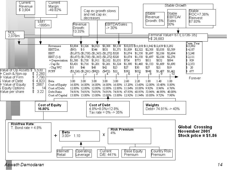
15
Valuing Global Crossing with Distress
Probability of distress Price of 8 year, 12% bond issued by Global Crossing = $ 653 Probability of distress = 13.53% a year Cumulative probability of survival over 10 years = ( )10 = 23.37% Distress sale value of equity Book value of capital = $14,531 million Distress sale value = 15% of book value = .15*14531 = $2,180 million Book value of debt = $7,647 million Distress sale value of equity = $ 0 Distress adjusted value of equity Value of Global Crossing = $3.22 (.2337) + $0.00 (.7663) = $0.75
10 = 23.37% Distress sale value of equity. Book value of capital = $14,531 million. Distress sale value = 15% of book value = .15*14531 = $2,180 million. Book value of debt = $7,647 million. Distress sale value of equity = $ 0. Distress adjusted value of equity. Value of Global Crossing = $3.22 (.2337) + $0.00 (.7663) = $0.75.")
16
Adjusted Present Value Model
In the adjusted present value approach, the value of the firm is written as the sum of the value of the firm without debt (the unlevered firm) and the effect of debt on firm value Firm Value = Unlevered Firm Value + (Tax Benefits of Debt - Expected Bankruptcy Cost from the Debt) The unlevered firm value can be estimated by discounting the free cashflows to the firm at the unlevered cost of equity The tax benefit of debt reflects the present value of the expected tax benefits. In its simplest form, Tax Benefit = Tax rate * Debt The expected bankruptcy cost is a function of the probability of bankruptcy and the cost of bankruptcy (direct as well as indirect) as a percent of firm value.
 and the effect of debt on firm value. Firm Value = Unlevered Firm Value + (Tax Benefits of Debt - Expected Bankruptcy Cost from the Debt) The unlevered firm value can be estimated by discounting the free cashflows to the firm at the unlevered cost of equity. The tax benefit of debt reflects the present value of the expected tax benefits. In its simplest form, Tax Benefit = Tax rate * Debt. The expected bankruptcy cost is a function of the probability of bankruptcy and the cost of bankruptcy (direct as well as indirect) as a percent of firm value.")
17
Excess Return Models You can present any discounted cashflow model in terms of excess returns, with the value being written as: Value = Capital Invested + Present value of excess returns on current investments + Present value of excess returns on future investments This model can be stated in terms of firm value (EVA) or equity value.
 or equity value.")
20
Relative Valuation What is it?: The value of any asset can be estimated by looking at how the market prices “similar” or ‘comparable” assets. Philosophical Basis: The intrinsic value of an asset is impossible (or close to impossible) to estimate. The value of an asset is whatever the market is willing to pay for it (based upon its characteristics) Information Needed: To do a relative valuation, you need an identical asset, or a group of comparable or similar assets a standardized measure of value (in equity, this is obtained by dividing the price by a common variable, such as earnings or book value) and if the assets are not perfectly comparable, variables to control for the differences Market Inefficiency: Pricing errors made across similar or comparable assets are easier to spot, easier to exploit and are much more quickly corrected. Most valuations on Wall Street are relative valuations, involving three components - a multiple, a set of comparable firms and a story. (In an informal survey of equity research reports that I did in 1998 and 1999, 92% of equity research reports could be categorized as relative valuations (though some had appendices with expected cash flows). Implicitly, you assume that markets are correct on average. (A logical follow-up is that equity research analysts must be much stronger believers in market efficiency than they claim to be, if their primary tools are multiples.
 to estimate. The value of an asset is whatever the market is willing to pay for it (based upon its characteristics) Information Needed: To do a relative valuation, you need. an identical asset, or a group of comparable or similar assets. a standardized measure of value (in equity, this is obtained by dividing the price by a common variable, such as earnings or book value) and if the assets are not perfectly comparable, variables to control for the differences. Market Inefficiency: Pricing errors made across similar or comparable assets are easier to spot, easier to exploit and are much more quickly corrected. Most valuations on Wall Street are relative valuations, involving three components - a multiple, a set of comparable firms and a story. (In an informal survey of equity research reports that I did in 1998 and 1999, 92% of equity research reports could be categorized as relative valuations (though some had appendices with expected cash flows). Implicitly, you assume that markets are correct on average. (A logical follow-up is that equity research analysts must be much stronger believers in market efficiency than they claim to be, if their primary tools are multiples.")
21
Variations on Multiples
Equity versus Firm Value Equity multiples (Price per share or Market value of equity) Firm value multiplies (Firm value or Enterprise value) Scaling variable Earnings (EPS, Net Income, EBIT, EBITDA) Book value (Book value of equity, Book value of assets, Book value of capital) Revenues Sector specific variables Base year Most recent financial year (Current) Last four quarters (Trailing) Average over last few years (Normalized) Expected future year (Forward) Comparables Sector Market
 Firm value multiplies (Firm value or Enterprise value) Scaling variable. Earnings (EPS, Net Income, EBIT, EBITDA) Book value (Book value of equity, Book value of assets, Book value of capital) Revenues. Sector specific variables. Base year. Most recent financial year (Current) Last four quarters (Trailing) Average over last few years (Normalized) Expected future year (Forward) Comparables. Sector. Market.")
22
Definitional Tests Is the multiple consistently defined?
Proposition 1: Both the value (the numerator) and the standardizing variable ( the denominator) should be to the same claimholders in the firm. In other words, the value of equity should be divided by equity earnings or equity book value, and firm value should be divided by firm earnings or book value. Is the multiple uniformally estimated? The variables used in defining the multiple should be estimated uniformly across assets in the “comparable firm” list. If earnings-based multiples are used, the accounting rules to measure earnings should be applied consistently across assets. The same rule applies with book-value based multiples.
 and the standardizing variable ( the denominator) should be to the same claimholders in the firm. In other words, the value of equity should be divided by equity earnings or equity book value, and firm value should be divided by firm earnings or book value. Is the multiple uniformally estimated The variables used in defining the multiple should be estimated uniformly across assets in the comparable firm list. If earnings-based multiples are used, the accounting rules to measure earnings should be applied consistently across assets. The same rule applies with book-value based multiples.")
23
An Example: Price Earnings Ratio: Definition
PE = Market Price per Share / Earnings per Share There are a number of variants on the basic PE ratio in use. They are based upon how the price and the earnings are defined. Price: is usually the current price is sometimes the average price for the year EPS: earnings per share in most recent financial year earnings per share in trailing 12 months (Trailing PE) forecasted earnings per share next year (Forward PE) forecasted earnings per share in future year
 forecasted earnings per share next year (Forward PE) forecasted earnings per share in future year.")
24
Descriptive Tests What is the average and standard deviation for this multiple, across the universe (market)? What is the median for this multiple? The median for this multiple is often a more reliable comparison point. How large are the outliers to the distribution, and how do we deal with the outliers? Throwing out the outliers may seem like an obvious solution, but if the outliers all lie on one side of the distribution (they usually are large positive numbers), this can lead to a biased estimate. Are there cases where the multiple cannot be estimated? Will ignoring these cases lead to a biased estimate of the multiple? How has this multiple changed over time?
, this can lead to a biased estimate. Are there cases where the multiple cannot be estimated Will ignoring these cases lead to a biased estimate of the multiple How has this multiple changed over time")
25
PE Ratio: Descriptive Statistics
This graph for all U.S. firms with data available on the Value Line CD ROM (contains about 7200 firms in the overall sample). Notice that the distributions are skewed to the left and that we have capped the PE ratios at 100….
. Notice that the distributions are skewed to the left and that we have capped the PE ratios at 100….")
26
PE: Deciphering the Distribution
Four things to note… Notice the number of firms that we have lost in the sample as we compute PE ratios. You lose even more firms as you go to forward PE, because you need analyst estimates of expected earnings per share to compute this. Any firms not followed by analysts will not have a forward PE… The means were computed without capping the PE ratios… the outliers (notice the maximum values for the ratios) push the average to almost twice the median. The median forward PE is higher than the trailing PE which is higher than the current PE…
 push the average to almost twice the median. The median forward PE is higher than the trailing PE which is higher than the current PE…")
27
8 Times EBITDA is not cheap…

28
Analytical Tests What are the fundamentals that determine and drive these multiples? Proposition 2: Embedded in every multiple are all of the variables that drive every discounted cash flow valuation - growth, risk and cash flow patterns. In fact, using a simple discounted cash flow model and basic algebra should yield the fundamentals that drive a multiple How do changes in these fundamentals change the multiple? The relationship between a fundamental (like growth) and a multiple (such as PE) is seldom linear. For example, if firm A has twice the growth rate of firm B, it will generally not trade at twice its PE ratio Proposition 3: It is impossible to properly compare firms on a multiple, if we do not know the nature of the relationship between fundamentals and the multiple.
 and a multiple (such as PE) is seldom linear. For example, if firm A has twice the growth rate of firm B, it will generally not trade at twice its PE ratio. Proposition 3: It is impossible to properly compare firms on a multiple, if we do not know the nature of the relationship between fundamentals and the multiple.")
29
Relative Value and Fundamentals
All multiples have their roots in fundamentals. A little algebra can take a discounted cash flow model and state it in terms of a multiple. This, in turn, allows us to find the fundamentals that drive each multiple: PE : Growth, Risk, Payout PBV: Growth, Risk, Payout, ROE PS: Growth, Risk, Payout, Net Margin. Every multiple has a companion variable, which more than any other variable drives that multiple. The companion variable for the multiples listed above are underlined. When comparing firms, this is the variable that you have to take the most care to control for. When people use multiples because they do not want to make the assumptions that DCF valuation entails, they are making the same assumptions implicitly.

30
What to control for... Multiple Variables that determine it…
PE Ratio Expected Growth, Risk, Payout Ratio PBV Ratio Return on Equity, Expected Growth, Risk, Payout PS Ratio Net Margin, Expected Growth, Risk, Payout Ratio EVV/EBITDA Expected Growth, Reinvestment rate, Cost of capital EV/ Sales Operating Margin, Expected Growth, Risk, Reinvestment

31
Application Tests Given the firm that we are valuing, what is a “comparable” firm? While traditional analysis is built on the premise that firms in the same sector are comparable firms, valuation theory would suggest that a comparable firm is one which is similar to the one being analyzed in terms of fundamentals. Proposition 4: There is no reason why a firm cannot be compared with another firm in a very different business, if the two firms have the same risk, growth and cash flow characteristics. Given the comparable firms, how do we adjust for differences across firms on the fundamentals? Proposition 5: It is impossible to find an exactly identical firm to the one you are valuing.

32
Comparing PE Ratios across a Sector

33
PE, Growth and Risk Dependent variable is: PE
R squared = 66.2% R squared (adjusted) = 63.1% Variable Coefficient SE t-ratio prob Constant Growth rate ≤ Emerging Market Emerging Market is a dummy: 1 if emerging market 0 if not
 = 63.1% Variable Coefficient SE t-ratio prob. Constant Growth rate ≤ Emerging Market Emerging Market is a dummy: 1 if emerging market. 0 if not.")
34
Is Telebras under valued?
Predicted PE = (.075) (1) = 8.35 At an actual price to earnings ratio of 8.9, Telebras is slightly overvalued.
 (1) = At an actual price to earnings ratio of 8.9, Telebras is slightly overvalued.")
35
PE Ratio without a constant - US Stocks
Tbe problem with a negative intercept in a regression is that predicted values for PE ratios can be negative. One way to get around this problem is to run the regression without a constant. There are two drawbacks. One is that the R squared is no longer comparable to the R-squared of a regular regression. The other is that the fit of your line (in terms of squared distances from the line) is not as good as the regular regression line.
 is not as good as the regular regression line.")
36
Relative Valuation: Choosing the Right Model

37
Contingent Claim (Option) Valuation
Options have several features They derive their value from an underlying asset, which has value The payoff on a call (put) option occurs only if the value of the underlying asset is greater (lesser) than an exercise price that is specified at the time the option is created. If this contingency does not occur, the option is worthless. They have a fixed life Any security that shares these features can be valued as an option. There are a lot of assets that have these characteristics that may not be categorized as options…. Option pricing models will do a better job of valuing these assets than traditional discounted cash flow models.
 option occurs only if the value of the underlying asset is greater (lesser) than an exercise price that is specified at the time the option is created. If this contingency does not occur, the option is worthless. They have a fixed life. Any security that shares these features can be valued as an option. There are a lot of assets that have these characteristics that may not be categorized as options…. Option pricing models will do a better job of valuing these assets than traditional discounted cash flow models.")
38
Option Payoff Diagrams
Shows the payoff diagram at expiration on call and put options. The essence of the options is that they have limited downside risk and significant upside potential. Any asset that has a payoff diagram that looks like this has option characteristics.

39
Underlying Theme: Searching for an Elusive Premium
Traditional discounted cashflow models under estimate the value of investments, where there are options embedded in the investments to Delay or defer making the investment (delay) Adjust or alter production schedules as price changes (flexibility) Expand into new markets or products at later stages in the process, based upon observing favorable outcomes at the early stages (expansion) Stop production or abandon investments if the outcomes are unfavorable at early stages (abandonment) Put another way, real option advocates believe that you should be paying a premium on discounted cashflow value estimates.
 Adjust or alter production schedules as price changes (flexibility) Expand into new markets or products at later stages in the process, based upon observing favorable outcomes at the early stages (expansion) Stop production or abandon investments if the outcomes are unfavorable at early stages (abandonment) Put another way, real option advocates believe that you should be paying a premium on discounted cashflow value estimates.")
40
Three Basic Questions When is there a real option embedded in a decision or an asset? There has to be a clearly defined underlying asset whose value changes over time in unpredictable ways. The payoffs on this asset (real option) have to be contingent on an specified event occurring within a finite period. When does that real option have significant economic value? For an option to have significant economic value, there has to be a restriction on competition in the event of the contingency. At the limit, real options are most valuable when you have exclusivity - you and only you can take advantage of the contingency. They become less valuable as the barriers to competition become less steep. Can that value be estimated using an option pricing model? The underlying asset is traded - this yield not only observable prices and volatility as inputs to option pricing models but allows for the possibility of creating replicating portfolios An active marketplace exists for the option itself. The cost of exercising the option is known with some degree of certaint
 have to be contingent on an specified event occurring within a finite period. When does that real option have significant economic value For an option to have significant economic value, there has to be a restriction on competition in the event of the contingency. At the limit, real options are most valuable when you have exclusivity - you and only you can take advantage of the contingency. They become less valuable as the barriers to competition become less steep. Can that value be estimated using an option pricing model The underlying asset is traded - this yield not only observable prices and volatility as inputs to option pricing models but allows for the possibility of creating replicating portfolios. An active marketplace exists for the option itself. The cost of exercising the option is known with some degree of certaint.")
41
Putting Natural Resource Options to the Test
The Option Test: Underlying Asset: Oil or gold in reserve Contingency: If value > Cost of development: Value - Dev Cost If value < Cost of development: 0 The Exclusivity Test: Natural resource reserves are limited (at least for the short term) It takes time and resources to develop new reserves The Option Pricing Test Underlying Asset: While the reserve or mine may not be traded, the commodity is. If we assume that we know the quantity with a fair degree of certainty, you can trade the underlying asset Option: Oil companies buy and sell reserves from each other regularly. Cost of Exercising the Option: This is the cost of developing a reserve. Given the experience that commodity companies have with this, they can estimate this cost with a fair degree of precision. Bottom Line: Real option pricing models work well with natural resource options.
 It takes time and resources to develop new reserves. The Option Pricing Test. Underlying Asset: While the reserve or mine may not be traded, the commodity is. If we assume that we know the quantity with a fair degree of certainty, you can trade the underlying asset. Option: Oil companies buy and sell reserves from each other regularly. Cost of Exercising the Option: This is the cost of developing a reserve. Given the experience that commodity companies have with this, they can estimate this cost with a fair degree of precision. Bottom Line: Real option pricing models work well with natural resource options.")
42
The Real Options Test: Patents and Technology
The Option Test: Underlying Asset: Product that would be generated by the patent Contingency: If PV of CFs from development > Cost of development: PV - Cost If PV of CFs from development < Cost of development: 0 The Exclusivity Test: Patents restrict competitors from developing similar products Patents do not restrict competitors from developing other products to treat the same disease. The Pricing Test Underlying Asset: Patents are not traded. Not only do you therefore have to estimate the present values and volatilities yourself, you cannot construct replicating positions or do arbitrage. Option: Patents are bought and sold, though not as frequently as oil reserves or mines. Cost of Exercising the Option: This is the cost of converting the patent for commercial production. Here, experience does help and drug firms can make fairly precise estimates of the cost. Bottom Line: Use real option pricing arguments with caution.

43
The Real Options Test for Growth (Expansion) Options
The Options Test Underlying Asset: Expansion Project Contingency If PV of CF from expansion > Expansion Cost: PV - Expansion Cost If PV of CF from expansion < Expansion Cost: 0 The Exclusivity Test Barriers may range from strong (exclusive licenses granted by the government) to weaker (brand name, knowledge of the market) to weakest (first mover). The Pricing Test Underlying Asset: As with patents, there is no trading in the underlying asset and you have to estimate value and volatility. Option: Licenses are sometimes bought and sold, but more diffuse expansion options are not. Cost of Exercising the Option: Not known with any precision and may itself evolve over time as the market evolves. Bottom Line: Using option pricing models to value expansion options will not only yield extremely noisy estimates, but may attach inappropriate premiums to discounted cashflow estimates.
 to weaker (brand name, knowledge of the market) to weakest (first mover). The Pricing Test. Underlying Asset: As with patents, there is no trading in the underlying asset and you have to estimate value and volatility. Option: Licenses are sometimes bought and sold, but more diffuse expansion options are not. Cost of Exercising the Option: Not known with any precision and may itself evolve over time as the market evolves. Bottom Line: Using option pricing models to value expansion options will not only yield extremely noisy estimates, but may attach inappropriate premiums to discounted cashflow estimates.")
44
Summarizing the Real Options Argument
There are real options everywhere. Most of them have no significant economic value because there is no exclusivity associated with using them. When options have significant economic value, the inputs needed to value them in a binomial model can be used in more traditional approaches (decision trees) to yield equivalent value. The real value from real options lies in Recognizing that building in flexibility and escape hatches into large decisions has value Insights we get on understanding how and why companies behave the way they do in investment analysis and capital structure choices.
 to yield equivalent value. The real value from real options lies in. Recognizing that building in flexibility and escape hatches into large decisions has value. Insights we get on understanding how and why companies behave the way they do in investment analysis and capital structure choices.")
46
Which approach should you use? Depends upon the asset being valued..

47
And the analyst doing the valuation….

Similar presentations


 –Residual income Model DCF and risidual income model are.>")


