1. Huffman code and Lossless Decomposition Prof. Sin-Min Lee Department of Computer Science

2. Data Compression Data discussed so far have used FIXED length for representation For data transfer (in particular), this method is inefficient. For speed and storage efficiencies, data symbols should use the minimum number of bits possible for representation.

3. Data Compression Methods Used For Compression: –Encode high probability symbols with fewer bits Shannon-Fano, Huffman, UNIX compact –Encode sequences of symbols with location of sequence in a dictionary PKZIP, ARC, GIF, UNIX compress, V.42bis –Lossy compression JPEG and MPEG

4. Data Compression Average code length Instead of the length of individual code symbols or words, we want to know the behavior of the complete information source

5. Data Compression Average code length Assume that symbols of a source alphabet {a 1,a 2, …,a M } are generated with probabilities p 1,p 2, …,p M P(a i ) = p i (i = 1, 2, …, M) Assume that each symbol of the source alphabet is encoded with codes of lengths l 1,l 2, …,l M

6. Data Compression Average code length Then the Average code length, L, of an information source is given by:

7. Data Compression Variable Length Bit Codings Rules: 1.Use minimum number of bits AND 2.No code is the prefix of another code AND 3.Enables left-to-right, unambiguous decoding

8. Data Compression Variable Length Bit Codings No code is a prefix of another –For example, can’t have ‘A’ map to 10 and ‘B’ map to 100, because 10 is a prefix (the start of) 100.

9. Data Compression Variable Length Bit Codings Enables left-to-right, unambiguous decoding –That is, if you see 10, you know it’s ‘A’, not the start of another character.

10. Data Compression Variable Length Bit Codings Suppose ‘A’ appears 50 times in text, but ‘B’ appears only 10 times ASCII coding assigns 8 bits per character, so total bits for ‘A’ and ‘B’ is 60 * 8 = 480 If ‘A’ gets a 4-bit code and ‘B’ gets a 12-bit code, total is 50 * 4 + 10 * 12 = 320

11. Data Compression Variable Length Bit Codings Example: Source Symbol PC1C1 C2C2 C3C3 C4C4 C5C5 C6C6 A0.60000000 B0.250110 0110 C0.110110 01111 D0.05111110111 010 Average code length = 1.75

12. Data Compression Variable Length Bit Codings Question: Is this the best that we can get?

13. Data Compression Huffman code –Constructed by using a code tree, but starting at the leaves –A compact code constructed using the binary Huffman code construction method

14. Data Compression Huffman code Algorithm ① Make a leaf node for each code symbol Add the generation probability of each symbol to the leaf node ② Take the two leaf nodes with the smallest probability and connect them into a new node Add 1 or 0 to each of the two branches The probability of the new node is the sum of the probabilities of the two connecting nodes ③ If there is only one node left, the code construction is completed. If not, go back to (2)

15. Data Compression Huffman code Example Character (or symbol) frequencies –A: 20% (.20) e.g., ‘A’ occurs 20 times in a 100 character document, 1000 times in a 5000 character document, etc. –B: 9% (.09) –C: 15% (.15) –D: 11% (.11) –E: 40% (.40) –F: 5% (.05) Also works if you use character counts Must know frequency of every character in the document

16. C.15 A.20 D.11 F.05 B.09 E.40 Huffman code Example Symbols and their associated frequencies. Now we combine the two least common symbols (those with the smallest frequencies) to make a new symbol string and corresponding frequency. Data Compression

17. C.15 A.20 D.11 F.05 BF.14 B.09 E.40 Data Compression Huffman code Example Here’s the result of combining symbols once. Now repeat until you’ve combined all the symbols into a single string.

18. C.15 A.20 D.11 F.05 BF.14 B.09 BFD.25 AC.35 E.40 ABCDF.60 ABCDEF 1.0 Data Compression Huffman code Example

19. Now assign 0s/1s to each branch Codes (reading from top to bottom) –A: 010 –B: 0000 –C: 011 –D: 001 –E: 1 –F: 0001 Note –None are prefixes of another ABCDEF 1.0 E.40 C.15 A.20 D.11 F.05 BF.14 AC.35 BFD.25 ABCDF.60 B.09 0 0 0 0 0 1 1 1 1 1 Data Compression Average Code Length = ?

20. Data Compression Huffman code There is no unique Huffman code –Assigning 0 and 1 to the branches is arbitrary –If there are more nodes with the same probability, it doesn ’ t matter how they are connected Every Huffman code has the same average code length!

21. Data Compression Huffman code Quiz: Symbols A, B, C, D, E, F are being produced by the information source with probabilities 0.3, 0.4, 0.06, 0.1, 0.1, 0.04 respectively. What is the binary Huffman code? 1)A = 00, B = 1, C = 0110, D = 0100, E = 0101, F = 0111 2)A = 00, B = 1, C = 01000, D = 011, E = 0101, F = 01001 3)A = 11, B = 0, C = 10111, D = 100, E = 1010, F = 10110

22. Data Compression Huffman code Applied extensively: Network data transfer MP3 audio format Gif image format HDTV Modelling algorithms

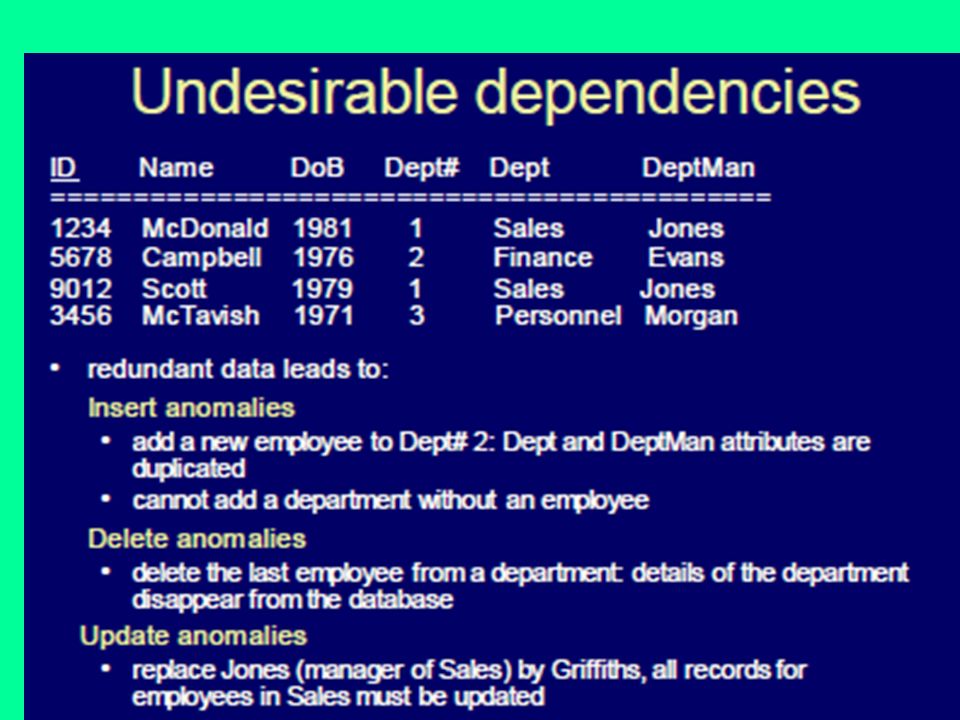
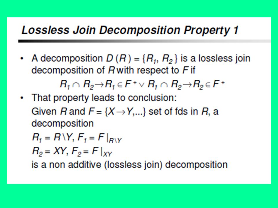
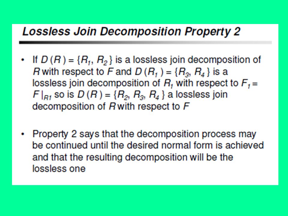
26. Loss-less Decompositions Definition: A decomposition of R into (R1, R2) is called lossless if, for all legal instance of r(R): r =  R1 (r )  R2 (r ) In other words, projecting on R1 and R2, and joining back, results in the relation you started with Rule: A decomposition of R into (R1, R2) is lossless, iff: R1 ∩ R2  R1 or R1 ∩ R2  R2 in F+.

28. Exercise

29. Answer

30. Dependency-preserving Decompositions Is it easy to check if the dependencies in F hold ? Okay as long as the dependencies can be checked in the same table. Consider R = (A, B, C), and F ={A  B, B  C} 1. Decompose into R1 = (A, B), and R2 = (A, C) Lossless ? Yes. But, makes it hard to check for B  C The data is in multiple tables. 2. On the other hand, R1 = (A, B), and R2 = (B, C), is both lossless and dependency-preserving Really ? What about A  C ? If we can check A  B, and B  C, A  C is implied.

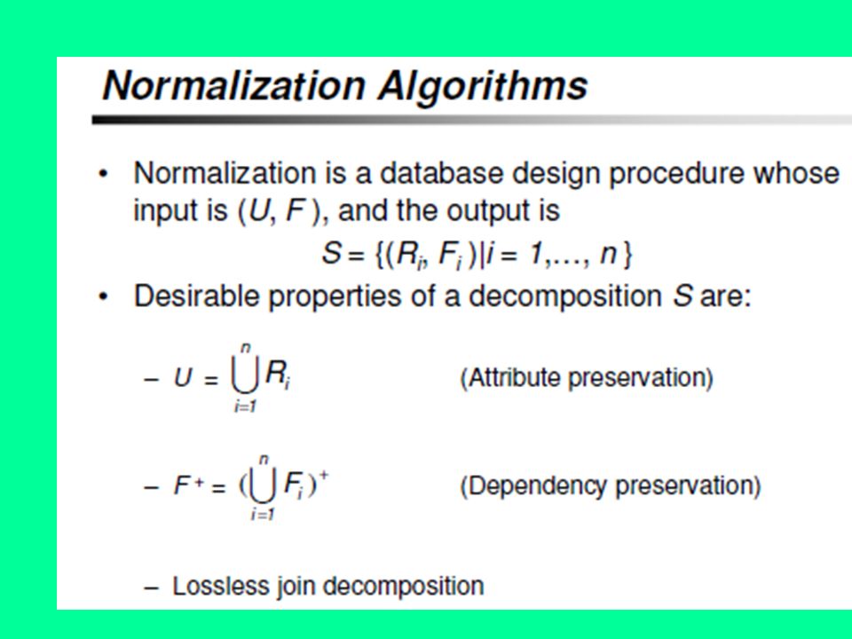
31. Dependency-preserving Decompositions Definition: Consider decomposition of R into R1, …, Rn. Let F i be the set of dependencies F + that include only attributes in R i. The decomposition is dependency preserving, if (F 1  F 2  …  F n ) + = F +

32. Example: Decompose Lossless but not dependency preserving Why ?

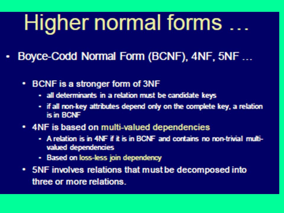
34. BCNF Given a relation schema R, and a set of functional dependencies F, if every FD, A  B, is either: 1. Trivial 2. A is a superkey of R Then, R is in BCNF (Boyce-Codd Normal Form) Why is BCNF good ?

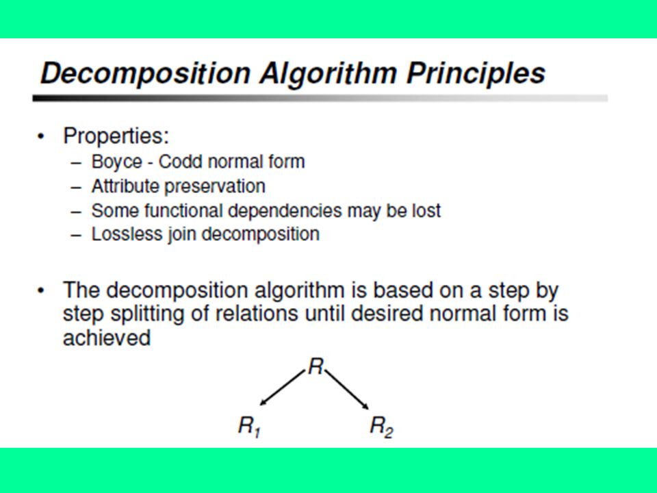
35. BCNF What if the schema is not in BCNF ? Decompose (split) the schema into two pieces. Careful: you want the decomposition to be lossless

38. Example

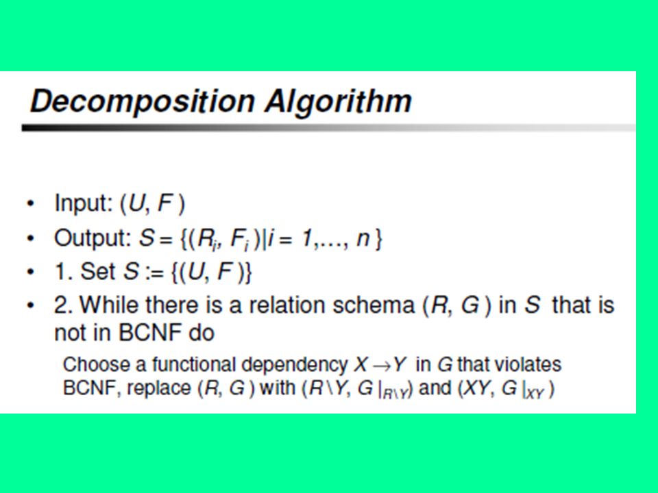
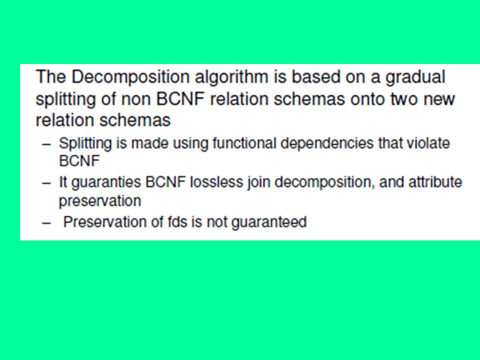
40. Achieving BCNF Schemas For all dependencies A  B in F+, check if A is a superkey By using attribute closure If not, then Choose a dependency in F+ that breaks the BCNF rules, say A  B Create R1 = A B Create R2 = A (R – B – A) Note that: R1 ∩ R2 = A and A  AB (= R1), so this is lossless decomposition Repeat for R1, and R2 By defining F1+ to be all dependencies in F that contain only attributes in R1 Similarly F2+

41. Example 1 B  C R = (A, B, C) F = {A  B, B  C} Candidate keys = {A} BCNF = No. B  C violates. R1 = (B, C) F1 = {B  C} Candidate keys = {B} BCNF = true R2 = (A, B) F2 = {A  B} Candidate keys = {A} BCNF = true

42. Example 2-1 A  B R = (A, B, C, D, E) F = {A  B, BC  D} Candidate keys = {ACE} BCNF = Violated by {A  B, BC  D} etc… R1 = (A, B) F1 = {A  B} Candidate keys = {A} BCNF = true R2 = (A, C, D, E) F2 = {AC  D} Candidate keys = {ACE} BCNF = false (AC  D) From A  B and BC  D by pseudo-transitivity AC  D R3 = (A, C, D) F3 = {AC  D} Candidate keys = {AC} BCNF = true R4 = (A, C, E) F4 = {} [[ only trivial ]] Candidate keys = {ACE} BCNF = true Dependency preservation ??? We can check: A  B (R1), AC  D (R3), but we lost BC  D So this is not a dependency -preserving decomposition

43. Example 2-2 BC  D R = (A, B, C, D, E) F = {A  B, BC  D} Candidate keys = {ACE} BCNF = Violated by {A  B, BC  D} etc… R1 = (B, C, D) F1 = {BC  D} Candidate keys = {BC} BCNF = true R2 = (B, C, A, E) F2 = {A  B} Candidate keys = {ACE} BCNF = false (A  B) A  B R3 = (A, B) F3 = {A  B} Candidate keys = {A} BCNF = true R4 = (A, C, E) F4 = {} [[ only trivial ]] Candidate keys = {ACE} BCNF = true Dependency preservation ??? We can check: BC  D (R1), A  B (R3), Dependency-preserving decomposition

44. Example 3 A  BC R = (A, B, C, D, E, H) F = {A  BC, E  HA} Candidate keys = {DE} BCNF = Violated by {A  BC} etc… R1 = (A, B, C) F1 = {A  BC} Candidate keys = {A} BCNF = true R2 = (A, D, E, H) F2 = {E  HA} Candidate keys = {DE} BCNF = false (E  HA) E  HA R3 = (E, H, A) F3 = {E  HA} Candidate keys = {E} BCNF = true R4 = (ED) F4 = {} [[ only trivial ]] Candidate keys = {DE} BCNF = true Dependency preservation ??? We can check: A  BC (R1), E  HA (R3), Dependency-preserving decomposition