Download presentation
Presentation is loading. Please wait.

1
Linear regression models

2
Purposes: To describe the linear relationship between two continuous variables, the response variable (y- axis) and a single predictor variable (x-axis) To determine how much of the variation in Y can be explained by the linear relationship with X and how much of this relationship remains unexplained To predict new values of Y from new values of X
 and a single predictor variable (x-axis) To determine how much of the variation in Y can be explained by the linear relationship with X and how much of this relationship remains unexplained To predict new values of Y from new values of X")
3
The linear regression model is: ß 0 = population intercept (when x i =0) ß 1 = population slope, measures the change in Y per unit change in X ε i = random or unexplained error associated with the i th observation.
 ß 1 = population slope, measures the change in Y per unit change in X ε i = random or unexplained error associated with the i th observation.")
4
Linear relationship Y X ß0ß0 ß1ß1 1.0

5
Linear models approximate non-linear functions over a limited domain extrapolation interpolation

6
μ yi = β o + β 1 *x i + є i x1x1 x2x2 μ y1 μ y2 yiyi y i pred y i –y pred = residual xixi Fitting data to a linear model

7
The residual The residual sum of squares

8
The “best fit” estimates are the values that minimize the residual sum of squares (RSS) between each observed value and the predicted value of the model
 between each observed value and the predicted value of the model")
9
Sum of squares Sun of cross products

10
Variance Covariance

11
Least-squares parameter estimates where

12
To solve the intercept

13
Variance of the error of regression

14
Variance components and Coefficient of determination

15
Coefficient of determination

16
Product-moment correlation coefficient

17
ANOVA table for regression SourceDegrees of freedom Sum of squaresMean square Expected mean square F ratio Regression 1 Residual n-2 Total n-1

18
Publication form of ANOVA table for regression Source Sum of Squaresdf Mean SquareFSig. Regression 11.4791 21.0440.00035 Residual 8.18215.545 Total 19.66116

19
Variance of estimated intercept

20
Variance of the slope estimator

21
Variance of the fitted value

22
Regression

23
Assumptions of regression The linear model correctly describes the functional relationship between X and Y The X variable is measured without error For a given value of X, the sampled Y values are independent with normally distributed errors Variances are constant along the regression line

24
Residual plot for species-area relationship

25
The influence function

26
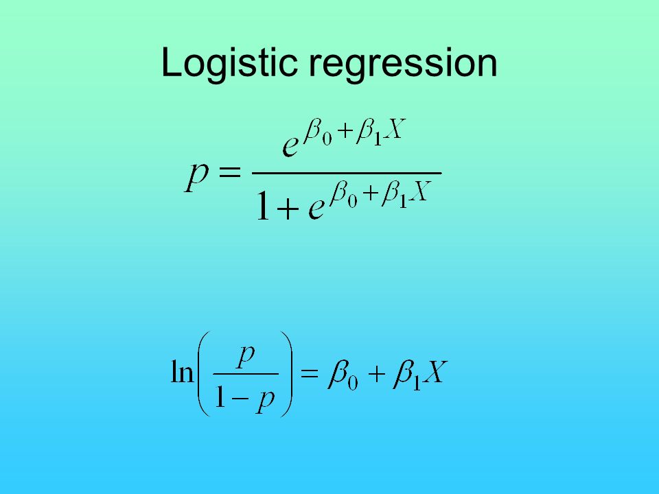
Logistic regression

28
Height vs. survival in Hypericum cumulicola

29
Multiple regression

30
Relative abundance of C 3 and C 4 plants Paruelo & Lauenroth (1996) Geographic distribution and the effects of climate variables on the relative abundance of a number of plant functional types (PFTs): shrubs, forbs, succulents, C 3 grasses and C 4 grasses.
 Geographic distribution and the effects of climate variables on the relative abundance of a number of plant functional types (PFTs): shrubs, forbs, succulents, C 3 grasses and C 4 grasses.")
31
data Relative abundance of PTFs (based on cover, biomass, and primary production) for each site Longitude Latitude Mean annual temperature Mean annual precipitation Winter (%) precipitation Summer (%) precipitation Biomes (grassland, shrubland) 73 sites across temperate central North America Response variablePredictor variables
 for each site Longitude Latitude Mean annual temperature Mean annual precipitation Winter (%) precipitation Summer (%) precipitation Biomes (grassland, shrubland) 73 sites across temperate central North America Response variablePredictor variables")
32
Box 6.1 Relative abundance transformed ln(dat+1) because positively skewed
 because positively skewed")
33
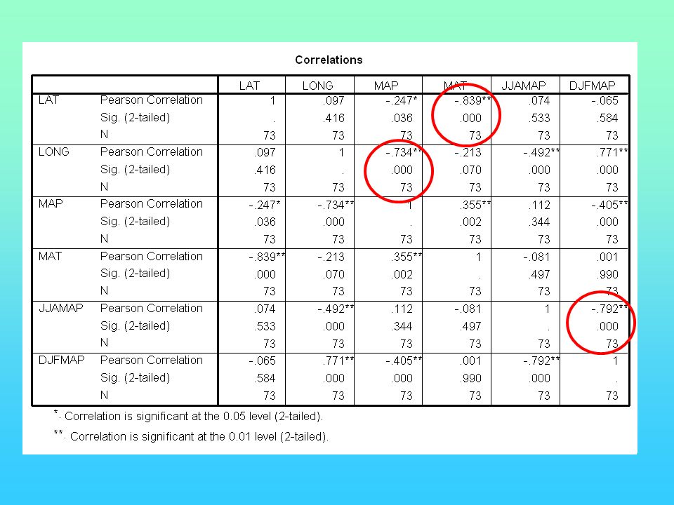
Collinearity Causes computational problems because it makes the determinant of the matrix of X-variables close to zero and matrix inversion basically involves dividing by the determinant (very sensitive to small differences in the numbers) Standard errors of the estimated regression slopes are inflated
 Standard errors of the estimated regression slopes are inflated")
34
Detecting collinearlity Check tolerance values Plot the variables Examine a matrix of correlation coefficients between predictor variables

35
Dealing with collinearity Omit predictor variables if they are highly correlated with other predictor variables that remain in the model

37
Additive model (log 10 C 3 )= β o + β 1 (lat)+ β 2 (long)+ β 3 (map)+ β 4 (mat)+ β 5 (JJAmap)+ β 6 (DJFmap) (lnC 3 )= β o + β 1 (lat)+ β 2 (long)+ β 3 (map)+ β 4 (mat)+ β 5 (JJAmap)+ β 6 (DJFmap) Adding 0.1
= β o + β 1 (lat)+ β 2 (long)+ β 3 (map)+ β 4 (mat)+ β 5 (JJAmap)+ β 6 (DJFmap) (lnC 3 )= β o + β 1 (lat)+ β 2 (long)+ β 3 (map)+ β 4 (mat)+ β 5 (JJAmap)+ β 6 (DJFmap) Adding 0.1")
38
Additive model (log 10 C 3 )= β o + β 1 (lat)+ β 2 (long)+ β 3 (map)+ β 4 (mat)+ β 5 (JJAmap)+ β 6 (DJFmap) (lnC 3 )= β o + β 1 (lat)+ β 2 (long)+ β 3 (map)+ β 4 (mat)+ β 5 (JJAmap)+ β 6 (DJFmap) Adding 0.1 Adding 1
= β o + β 1 (lat)+ β 2 (long)+ β 3 (map)+ β 4 (mat)+ β 5 (JJAmap)+ β 6 (DJFmap) (lnC 3 )= β o + β 1 (lat)+ β 2 (long)+ β 3 (map)+ β 4 (mat)+ β 5 (JJAmap)+ β 6 (DJFmap) Adding 0.1 Adding 1")
39
(lnC 3 )= β o + β 1 (lat)+ β 2 (long)+ β 3 (latxlong) After centering both lat and long
= β o + β 1 (lat)+ β 2 (long)+ β 3 (latxlong) After centering both lat and long")
40
If we omit the interaction and refit the model, the partial regression slope for latitude changes The collinearity problems disappear

42
R 2 =0.514

43
Matrix algebra approach to OLS estimation of multiple regression models Y=bX+ε X’Xb=X’Y b=(X’X) -1 (X’Y)
 -1 (X’Y)")
44
The forward selection is

45
The backward selection is

46
Adjusted r 2

47
Akaike information criteria

48
Bayesian information criteria

49
Hierarchical partitioning and model selection No predmodelr2r2 Adjr 2 CpCp AICSchwarz BIC 1 Lon 0.00005-0.014072.89-159.90-155.32 1 Lat 0.46180.45427.37-205.12-200.54 1 Lon x Lat 0.0062-0.007872.01-160.35-155.77 2 Lon + Lat 0.46710.45198.61-203.85-196.98 3 Long +Lat + Lon x Lat 0.51370.49264-208.53-199.67

Similar presentations


 Correlation: No variables are considered.>")


