1. CSS Data Warehousing for BS(CS) Lecture 1-2: DW & Need for DW Khurram Shahzad mks@ciitlahore.edu.pk Department of Computer Science

2. 2 Course Objectives At the end of the course you will (hopefully) be able to answer the questions  Why exactly the world needs a data warehouse?  How DW differs from traditional databases and RDBMS?  Where does OLAP stands in the DW picture?  What are different DW and OLAP models/schemas? How to implement and test these?  How to perform ETL? What is data cleansing? How to perform it? What are the famous algorithms?  Which different DW architectures have been reported in the literature? What are their strengths and weaknesses?  What latest areas of research and development are stemming out of DW domain?

3. 3 Course Material Course Book  Paulraj Ponniah, Data Warehousing Fundamentals, John Wiley & Sons Inc., NY. Reference Books  W.H. Inmon, Building the Data Warehouse (Second Edition), John Wiley & Sons Inc., NY.  Ralph Kimball and Margy Ross, The Data Warehouse Toolkit (Second Edition), John Wiley & Sons Inc., NY.

4. 4 Assignments Implementation/Research on important concepts. To be submitted in groups of 2 students. Include 1. Modeling and Benchmarking of multiple warehouse schemas 2. Implementation of an efficient OLAP cube generation algorithm 3. Data cleansing and transformation of legacy data 4. Literature Review paper on View Consistency Mechanisms in Data Warehouse Index design optimization Advance DW Applications May add a couple more

5. 5 Lab Work Lab Exercises. To be submitted individually

6. 6 Course Introduction What this course is about?  Decision Support Cycle Planning – Designing – Developing - Optimizing – Utilizing

7. 7 Course Introduction Information SourcesData Warehouse Server (Tier 1) OLAP Servers (Tier 2) Clients (Tier 3) Operational DB’s Semistructured Sources extract transform load refresh etc. Data Marts Data Warehouse e.g., MOLAP e.g., ROLAP serve Analysis Query/Reporting Data Mining serve

8. 8 Operational computer systems did provide information to run day-to-day operations, and answer’s daily questions, but… Also called online transactional processing system (OLTP) Data is read or manipulated with each transaction Transactions/queries are simple, and easy to write Usually for middle management Examples  Sales systems  Hotel reservation systems  COMSIS  HRM Applications  Etc. Operational Sources (OLTP’s)

9. 9 Typical decision queries Data set are mounting everywhere, but not useful for decision support Decision-making require complex questions from integrated data. Enterprise wide data is desired Decision makers want to know:  Where to build new oil warehouse?  Which market they should strengthen?  Which customer groups are most profitable?  How much is the total sale by month/ year/ quarter for each offices?  Is there any relation between promotion campaigns and sales growth? Can OLTP answer all such questions,  efficiently?

10. 10 Information crisis * Integrated  Must have a single, enterprise-wide view Data Integrity  Information must be accurate and must conform to business rules Accessible  Easily accessible with intuitive access paths and responsive for analysis Credible  Every business factor must have one and only one value Timely  Information must be available within the stipulated time frame * Paulraj 2001.

11. 11 Data Driven-DSS * * Farooq, lecture slides for ‘Data Warehouse’ course

12. 12 Failure of old DSS Inability to provide strategic information IT receive too many ad hoc requests, so large over load Requests are not only numerous, they change overtime For more understanding more reports Users are in spiral of reports Users have to depend on IT for information Can't provide enough performance, slow Strategic information have to be flexible and conductive

13. 13 OLTP vs. DSS Trait OLTP DSS User Middle management Executives, decision-makers Function For day-to-day operations For analysis & decision support DB (modeling) E-R based, after normalization Star oriented schemas Data Current, Isolated Archived, derived, summarized Unit of work Transactions Complex query Access, type DML, read Read Access frequency Very high Medium to Low Records accessed Tens to Hundreds Thousands to Millions Quantity of users Thousands Very small amount Usage Predictable, repetitive Ad hoc, random, heuristic based DB size 100 MB-GB 100GB-TB Response time Sub-seconds Up-to min.s

14. 14 Expectations of new soln. DB designed for analytical tasks Data from multiple applications Easy to use Ability of what-if analysis Read-intensive data usage Direct interaction with system, without IT assistance Periodical updating contents & stable Current & historical data Ability for users to initiate reports

15. 15 DW meets expectations Provides enterprise view Current & historical data available Decision-transaction possible without affecting operational source Reliable source of information Ability for users to initiate reports Acts as a data source for all analytical applications

16. 16 Definition of DW Inmon defined “A DW is a subject-oriented, integrated, non-volatile, time-variant collection of data in favor of decision-making”. Kelly said “Separate available, integrated, time-stamped, subject-oriented, non- volatile, accessible” Four properties of DW

17. 17 Subject-oriented In operational sources data is organized by applications, or business processes. In DW subject is the organization method Subjects vary with enterprise These are critical factors, that affect performance Example of Manufacturing Company  Sales  Shipment  Inventory etc

18. 18 Integrated Data Data comes from several applications Problems of integration comes into play  File layout, encoding, field names, systems, schema, data heterogeneity are the issues  Bank example, variance: naming convention, attributes for data item, account no, account type, size, currency In addition to internal, external data sources  External companies data sharing  Websites  Others Removal of inconsistency So process of extraction, transformation & loading

19. 19 Time variant Operational data has current values Comparative analysis is one of the best techniques for business performance evaluation Time is critical factor for comparative analysis Every data structure in DW contains time element In order to promote product in certain, analyst has to know about current and historical values The advantages are  Allows for analysis of the past  Relates information to the present  Enables forecasts for the future

20. 20 Non-volatile Data from operational systems are moved into DW after specific intervals Data is persistent/ not removed i.e. non volatile Every business transaction don’t update in DW Data from DW is not deleted Data is neither changed by individual transactions Properties summary Subject Oriented Organized along the lines of the subjects of the corporation. Typical subjects are customer, product, vendor and transaction. Time-Variant Every record in the data warehouse has some form of time variancy attached to it. Non-Volatile Refers to the inability of data to be updated. Every record in the data warehouse is time stamped in one form or another.

21. 21 Lecture 2 DW Architecture & Dimension Modeling Khurram Shahzad mks@ciitlahore.edu.pk

22. 22 Agenda Data Warehouse architecture & building blocks ER modeling review Need for Dimensional Modeling Dimensional modeling & its inside Comparison of ER with dimensional

23. 23 Architecture of DW Information SourcesData Warehouse Server (Tier 1) OLAP Servers (Tier 2) Clients (Tier 3) Operational DB’s Semistructured Sources extract transform load refresh Data Marts Data Warehouse e.g., MOLAP e.g., ROLAP serve Analysis Query/Reporting Data Mining serve Staging area

24. 24 Components Major components  Source data component  Data staging component  Information delivery component  Metadata component  Management and control component

25. 25 1. Source Data Components Source data can be grouped into 4 components  Production data Comes from operational systems of enterprise Some segments are selected from it Narrow scope, e.g. order details  Internal data Private datasheet, documents, customer profiles etc. E.g. Customer profiles for specific offering Special strategies to transform ‘it’ to DW (text document)  Archived data Old data is archived DW have snapshots of historical data  External data Executives depend upon external sources E.g. market data of competitors, car rental require new manufacturing. Define conversion

26. 26 Architecture of DW Information SourcesData Warehouse Server (Tier 1) OLAP Servers (Tier 2) Clients (Tier 3) Operational DB’s Semistructured Sources extract transform load refresh Data Marts Data Warehouse e.g., MOLAP e.g., ROLAP serve Analysis Query/Reporting Data Mining serve Staging area

27. 27 2. Data Staging Components After data is extracted, data is to be prepared Data extracted from sources needs to be changed, converted and made ready in suitable format Three major functions to make data ready  Extract  Transform  Load Staging area provides a place and area with a set of functions to  Clean  Change  Combine  Convert

28. 28 Architecture of DW Information SourcesData Warehouse Server (Tier 1) OLAP Servers (Tier 2) Clients (Tier 3) Operational DB’s Semistructured Sources extract transform load refresh Data Marts Data Warehouse e.g., MOLAP e.g., ROLAP serve Analysis Query/Reporting Data Mining serve Staging area

29. 29 3. Data Storage Components Separate repository Data structured for efficient processing Redundancy is increased Updated after specific periods Only read-only

30. 30 Architecture of DW Information SourcesData Warehouse Server (Tier 1) OLAP Servers (Tier 2) Clients (Tier 3) Operational DB’s Semistructured Sources extract transform load refresh Data Marts Data Warehouse e.g., MOLAP e.g., ROLAP serve Analysis Query/Reporting Data Mining serve Staging area

31. 31 4. Information Delivery Component Authentication issues Active monitoring services  Performance, DBA note selected aggregates to change storage  User performance  Aggregate awareness  E.g. mining, OLAP etc

32. 32 DW Design

33. 33 Designing DW Information SourcesData Warehouse Server (Tier 1) OLAP Servers (Tier 2) Clients (Tier 3) Operational DB’s Semistructured Sources extract transform load refresh Data Marts Data Warehouse e.g., MOLAP e.g., ROLAP serve Analysis Query/Reporting Data Mining serve Staging area

34. 34 Background (ER Modeling) For ER modeling, entities are collected from the environment Each entity act as a table Success reasons  Normalized after ER, since it removes redundancy (to handle update/delete anomalies) But number of tables is increased  Is useful for fast access of small amount of data

35. ER Drawbacks for DW / Need of Dimensional Modeling  ER Hard to remember, due to increased number of tables  Complex for queries with multiple tables (table joins)  Conventional RDBMS optimized for small number of tables whereas large number of tables might be required in DW  Ideally no calculated attributes  The DW does not require to update data like in OLTP system so there is no need of normalization  OLAP is not the only purpose of DW, we need a model that facilitate integration of data, data mining, historically consolidated data.  Efficient indexing scheme to avoid screening of all data De-Normalization (in DW)  Add primary key  Direct relationships  Re-introduce redundancy 35

36. 36 Dimensional Modeling Dimensional Modeling focuses subject- orientation, critical factors of business Critical factors are stored in facts Redundancy is no problem, achieve efficiency Logical design technique for high performance Is the modeling technique for storage

37. Dimensional Modeling (cont.) Two important concepts  Fact Numeric measurements, represent business activity/event Are pre-computed, redundant Example: Profit, quantity sold  Dimension Qualifying characteristics, perspective to a fact Example: date (Date, month, quarter, year) 37

38. 38 Dimensional Modeling (cont.) Facts are stored in fact table Dimensions are represented by dimension tables Dimensions are degrees in which facts can be judged Each fact is surrounded by dimension tables Looks like a star so called Star Schema

39. 39 Example TIME time_key (PK) SQL_date day_of_week month STORE store_key (PK) store_ID store_name address district floor_type CLERK clerk_key (PK) clerk_id clerk_name clerk_grade PRODUCT product_key (PK) SKU description brand category CUSTOMER customer_key (PK) customer_name purchase_profile credit_profile address PROMOTION promotion_key (PK) promotion_name price_type ad_type FACT time_key (FK) store_key (FK) clerk_key (FK) product_key (FK) customer_key (FK) promotion_key (FK) dollars_sold units_sold dollars_cost

40. 40 Inside Dimensional Modeling Inside Dimension table  Key attribute of dimension table, for identification  Large no of columns, wide table  Non-calculated attributes, textual attributes  Attributes are not directly related  Un-normalized in Star schema  Ability to drill-down and drill-up are two ways of exploiting dimensions  Can have multiple hierarchies  Relatively small number of records

41. 41 Inside Dimensional Modeling Have two types of attributes  Key attributes, for connections  Facts Inside fact table  Concatenated key  Grain or level of data identified  Large number of records  Limited attributes  Sparse data set  Degenerate dimensions (order number  Average products per order) Fact-less fact table

42. 42 Star Schema Keys Primary keys  Identifying attribute in dimension table  Relationship attributes combine together to form P.K Surrogate keys  Replacement of primary key  System generated Foreign keys  Collection of primary keys of dimension tables Primary key to fact table  System generated  Collection of P.Ks

43. 43 Advantage of Star Schema Ease for users to understand Optimized for navigation (less joins  fast) Most suitable for query processing Karen Corral, et al. (2006) The impact of alternative diagrams on the accuracy of recall: A comparison of star-schema diagrams and entity-relationship diagrams, Decision Support Systems, 42(1), 450-468.

44. Normalization [1] “It is the process of decomposing the relational table in smaller tables.” Normalization Goals: 1. Remove data redundancy 2. Storing only related data in a table (data dependency makes sense) 5 Normal Forms The decomposition must be lossless 44

45. 1 st Normal Form [2] “A relation is in first normal form if and only if every attribute is single-valued for each tuple” 45 STU_IDSTU_NAMEMAJORCREDITSCATEGORY S1001Tom SmithHistory90Comp S1003Mary JonesMath95Elective S1006Edward Burns CSC, Math15Comp, Elective S1010Mary JonesArt, English63Elective, Elective S1060John SmithCSC25Comp

46. 1 st Normal Form (Cont.) 46 STU_IDSTU_NAMEMAJORCREDITSCATEGORY S1001Tom SmithHistory90Comp S1003Mary JonesMath95Elective S1006Edward Burns CSC15Comp S1006Edward Burns Math15Elective S1010Mary JonesArt63Elective S1010Mary JonesEnglish63Comp S1060John SmithCSC25Comp

47. Another Example (composite key: SID, Course) [1] 47

48. 1st Normal Form Anomalies [1] Update anomaly: Need to update all six rows for student with ID=1if we want to change his location from Islamabad to Karachi Delete anomaly: Deleting the information about a student who has graduated will remove all of his information from the database Insert anomaly: For inserting the information about a student, that student must be registered in a course 48

49. Solution  2 nd Normal Form “A relation is in second normal form if and only if it is in first normal form and all the nonkey attributes are fully functional dependent on the key” [2] In previous example, functional dependencies [1] SID —> campus Campus  degree 49

50. Example in 2 nd Normal Form [1] 50

51. Anomalies [1] Insert Anomaly: Can not enter a program for example PhD for Peshawar campus unless a student get registered Delete Anomaly: Deleting a row from “Registration” table will delete all information about a student as well as degree program 51

52. Solution  3 rd Normal Form “A relation is in third normal form if it is in second normal form and nonkey attribute is transitively dependent on the key” [2] In previous example: [1] Campus  degree 52

53. Example in 3 rd Normal Form [1] 53

54. Denormalization [1] “Denormanlization is the process” to selectively transforms the normalized relations in to un-normalized form with the intention to “reduce query processing time” The purpose is to reduce the number of tables to avoid the number of joins in a query 54

55. Five techniques to denormalize relations [1] Collapsing tables Pre-joining Splitting tables (horizontal, vertical) Adding redundant columns Derived attributes 55

56. Collapsing tables (one-to-one) [1] 56 For example, Student_ID, Gender in Table 1 and Student_ID, Degree in Table 2

57. Pre-joining [1] 57

58. Splitting tables [1] 58

59. Redundant columns [1] 59

60. Updates to Dimension Tables 60

61. Updates to Dimension Tables (Cont.) Type-I changes: correction of errors, e.g., customer name changes from Sulman Khan to Salman Khan Solution to type-I updates:  Simply update the corresponding attribute/attributes. There is no need to preserve their old values 61

62. Updates to Dimension Tables (Cont.) Type 2 changes: preserving history For example change in “address” of a customer, but the user wants to see orders by geographic location then you can not simply update the address by replacing old value with new value, you need to preserve the history (old value) as well as need to insert new value 62

63. Updates to Dimension Tables (Cont.) Proposed solution: 63

64. Updates to Dimension Tables (Cont.) Type 3 changes: When you want to compare old and new values of attributes for a given period Please note that in Type 2 changes the old values and new values were not comparable before or after the cut-off date (when the address was changed) 64

65. Updates to Dimension Tables (Cont.) 65 Solution: Add a new column of attribute

66. Updates to Dimension Tables (Cont.) 66 What if we want to keep a whole history of changes? Should we add large number of attributes to tackle it?

67. Rapidly Changing Dimension When dimension’s records/rows are very large in numbers and changes are required frequently then Type-II change handling is not recommended It is recommended to make a separate table of rapidly changing attributes 67

68. Rapidly Changing Dimension (Cont.) “For example, an important attribute for customers might be their account status (good, late, very late, in arrears, suspended), and the history of their account status” [4] “If this attribute is kept in the customer dimension table and a type 2 change is made each time a customer's status changes, an entire row is added only to track this one attribute” [4] “The solution is to create a separate account_status dimension with five members to represent the account states” [4] and join this new table or dimension to the fact table. 68

69. Example 69

70. Junk Dimensions Sometimes there are some informative flags and texts in the source system, e.g., yes/no flags, textual codes, etc. If such flags are important then make their own dimension to save the storage space 70

71. Junk Dimension Example [3] 71

72. Junk Dimension Example (Cont.) [3] 72

73. The Snowflake Schema Snowflacking involves normalization of dimensions in Star Schema Reasons: To save storage space To optimize some specific quires (for attributes with low cardinality) 73

74. Example 1 of Snowflake Schema 74

75. Example 2 of Snowflake Schema 75

76. Aggregate Fact Tables Use aggregate fact tables when too many rows of fact tables are involved in making summary of required results Objective is to reduce query processing time 76

77. Example 77 Total Possible Rows = 1825 * 300 * 4000 * 1 = 2 billion

78. Solution Make aggregate fact tables, because you might be summing some dimension and some might not then why we should store the dimensions that do not need highest level of granularity of details. For example: Sales of a product in a year OR total number of items sold by category on daily basis 78

79. A way of making aggregates Example: 79

80. Making Aggregates But first determine what is required from your data warehouse then make aggregates 80

81. Families of Stars 81

82. Families of Stars (Cont.) Transaction (day to day) and snapshot tables (data after some specific intervals) 82

83. Families of Stars (Cont.) Core and custom tables 83

84. Families of Stars (Cont.) Conformed Dimension: The attributes of a dimension must have the same meaning for all those fact tables with which the dimension is connected. 84

85. Extract, Transform, Load (ETL) Extract only relevant data from the internal source systems or external systems, instead of dumping all data (“data junkhouse”) The ETL completion can take up to 50-70% of your total effort while developing a data warehouse. These ETL efforts depends on various factors which will be elaborated as we proceed in our lectures regarding ETL. 85

86. Major steps in ETL 86

87. Data Extraction Data can be extracted using third party tools or in-house programs or scripts Data extraction issues: 1. Identify sources 2. Method of extraction for each source (manual, automated) 3. When and how much frequently data will be extracted for each source 4. Time window 5. Sequencing of extraction processes 87

88. How data is stored in operational systems Current value: Values continue to changes as daily transactions are performed. We need to monitor these changes to maintain history for decision making process, e.g., bank balance, customer address, etc. Periodic status: sometimes the history of changes is maintained in the source system 88

89. Example 89

90. Data Extraction Method Static data extraction: 1. Extract the data at a certain time point. 2. It will include all transient data and periodic data along with its time/date status at the extraction time point 3. Used for initial data loading Data of revisions 1. Data is loaded in increments thus preserving history of both changing and periodic data 90

91. Incremental data extraction Immediate data extraction: involves data extraction in real time. Possible options: 1. Capture through transactions logs 2. Make triggers/Stored procedures 3. Capture via source application 4. Capture on the basis of time and date stamps 5. Capture by comparing files 91

92. Data Transformation Transformation means to integrate or consolidate data from various sources Major tasks: 1. Format conversions (change in data type, length) 2. Decoding of fields (1,0  male, female) 3. Calculated and derived values (units sold, price, cost  profit) 4. Splitting of single fields (House no 10, ABC Road, 54000, Lahore, Punjab, Pakistan) 5. Merging of information (information from different sources regarding any entity, attribute) 6. Character set conversion 92

93. Data Transformation (Cont.) 8. Conversion of unit of measures 9. Date/time conversion 10. Key restructuring 11. De-duplication 12. Entity identification 13. Multiple source problem 93

94. Data Loading Determine when (time) and how (as a whole or in chunks) to load data Four modes to load data 1. Load: removes old data if available otherwise load data 2. Append: The old data is not removed, the new data is appended with the old data 3. Destructive Merge: If primary key of the new record matched with the primary key of and old record then update old record 4. Constructive Merge: If primary key of the new record matched with the primary key of and old record then do not update old record just add the new record and mark it as superseding record

95. Data Loading (Cont.) Data Refresh Vs. Data Update Full refresh reloads whole data after deleting old data and data updates are used to update the changing attributes

96. Data Loading (Cont.) Loading for dimensional tables: You need to define a mapping between source system key and system generated key in data warehouse, otherwise you will not be able to load/update data correctly

97. Data Loading (Cont.) Updates to dimension table

98. Data Quality Management It is important to ensure that the data is correct to make right decisions Imagine the user working on operational system is entering wrong regions’ codes of customers. Imagine that the relevant business has never sent an invoice using these regions codes (so they are ignorant). But what will happen if the data warehouse will use these codes to make decisions? You need to put proper time and effort to ensure data quality

99. Data Quality What is Data: An abstraction/representation/ description of something in reality What is Data Quality: Accuracy + Data must serve its purpose/user expectations

100. Indicators of quality of data Accuracy: Correct information, e.g., address of the customer is correct Domain Integrity: Allowable values, e.g., male/female Consistency: The content and its form is same across all source system, e.g., product code of a product ABC in one system is 1234 then in other system it must be 1234 for that particular product

101. Indicators of quality of data (Cont.) Redundancy: Data is not redundant, if for some reason for example efficiency the data is redundant then it must be identified accordingly Completeness: There are no missing values in any field Conformance to Business rules: Values are according to the business constraints, e.g., loan issued cannot be negative Well defined structure: Whenever the data item can be divided in components it must be stored in terms of components/well structure, e.g., Muhammad Ahmed Khan can be structured as first name, middle name, last name. Similar is the case with addresses

102. Indicators of quality of data (Cont.) Data Anomaly: Fields must contain that value for which it was created, e.g., State filed cannot take the city name Proper Naming convention Timely: timely data updates as required by user Usefulness: The data elements in data warehouse must be useful and fulfill the requirements of the users otherwise data warehouse is not of any value

103. Indicators of quality of data (Cont.) Entity and Referential Integrity: Entity integrity means every table must have a primary key and it must be unique and not null. Referential integrity enforces parent child relationship between tables, you can not insert a record in child table unless you have a corresponding record in parent table

104. SQL Server Integration Services (SSIS)

105. Problems due to quality of data Businesses ranked data quality as the biggest problem during data warehouse designing and usage

106. Possible causes of low quality data Dummy values: For example, to pass a check on postal code, entering dummy or not precise information such as 4444 (dummy) or 54000 for all regions of Lahore Absence of data values: For example not a complete address Unofficial use of field: For example writing comments in the contact field of the customer

107. Possible causes of low quality data Cryptic Information: At one time operation system was using ‘R’ for “remove” then later for “reduced” and some other time point for “recovery” Contradicting values: compatible fields must not contradict, e.g., two fileds ZIP code and City can have values 54000 and Lahore but not some other city name for ZIP code 54000

108. Possible causes of low quality data Violation of business rule: Issued load is negative Reused primary keys: For example, a business has 2 digit primary key. It can have maximum 100 customers. When a 101th customer comes the business might archive the old customers and assign the new customer a primary key from the start. It might not be a problem for the operation system but you need to resolve such issues because DW keeps historical data.

109. Possible causes of low quality data Non-unique identifiers: For example different product codes in different departments Inconsistent values: one system is using male/female to represent gender while other system is using 1/0 Incorrect values: Product Code: 466, Product Name: “Crystal vas”, Height:”500 inch”. It means that product and height values are not compatible. Either product name or height is wrong or maybe the product code as well

110. Possible causes of low quality data Erroneous integration: A person might be a buyer or seller to your business. Your customer table might be storing such person with ID 222 while in seller table it might be 500. In data warehouse you might need to integrate this information. The persons with IDs 222 in both tables might not be same

111. Sources of data pollution System migration or conversions: For example, from manual system  Flat files  Hierarchal databases  relational databases…. Integration of heterogeneous systems: More heterogeneity means more problems Poor database design: For example lack of business rules, lack of entity and referential integrity

112. Sources of data pollution (Cont.) Incomplete data entry: For example, no city information Wrong information during entry: For example United Kingdom  Unted Kingdom

113. Data Cleansing

114. Examples of data cleansing tools Data Ladder, http://www.dataladder.com/products.htmlhttp://www.dataladder.com/products.html Human Inference, http://www.humaninference.com/master-data-management/data- quality/data-cleansing Google Refine, http://code.google.com/p/google-refine/ Wrangler http://vis.stanford.edu/wrangler/ Text Pipe Pro http://www.datamystic.com/textpipe.html#.UKjm9eQ3vyo

115. Information Supply It deals with how you will provide information to the users of the data warehouse. It must be easy to use, appealing, and insightful For successful data warehouse you need to identify users, and when, what, where, and how (in which form) they need information

116. Data warehouse modes of usage Verification mode: The users interact with the system to prove or disprove a hypothesis Discovery mode: Without any prior hypothesis. The intention is to discover new things or knowledge about the business. The data mining techniques are used here.

117. Approaches of interaction with data warehouse Informational approach: 1. With queries and reporting tools 2. The data might be summarized 3. Can perform statistical analysis by using current and historical data Analytical approach: 1. Used for analysis in terms of drill-up, drill-down, slice, and dice Data Mining approach 1. Used for knowledge discovery or hidden patterns

118. Classes of users We need to identify the classes of users in order to get firm basis what and how to provide information to them A typical example of classifying users

119. User classes (cont.) Naive users Regular users: daily users but cannot make queries and reports themselves. They need query templates and predefined reports Power users: Technically sound users, who can make queries, reports, scripts, import and export data themselves

120. User classes from other perspective High-level Executives and Managers: Need standard pre-processed reports to make strategic decisions Technical Analysts: complex analysis, statistical analysis, drill-down, slice, dice Business Analysts: comfortable with technology but cannot make queries, can modify reports to get information from different angles. Business-Oriented users: Predefined GUIs, and might be support for some ad-hoc queries

121. The ways of interaction Preprocessed reports: routine reports which are delivered at some specific interval Predefined queries and templates: The users can use own parameters with predefined queries templates and reports with predefined format Limited ad-hoc access: few and simple queries which are developed from scratch Complex ad-hoc access: complicated queries and analysis. Can be used as a basis for predefined reports and queries

122. Information delivery framework

123. Online Analytical Processing (OLAP) used for fast and complex analysis on data warehouse It is not a database design technique but is only a category of applications Definition by Dr. E. F. Codd “On-Line Analytical Processing (OLAP) is a category of software technology that enables analysts, managers and executives to gain insight into data through fast, consistent, interactive access in a wide variety of possible views of information that has been transformed from raw data to reflect the real dimensionality of the enterprise as understood by the user.” So what is the difference between data warehouse and OLAP?

124. OLAP (cont.)

125. What is the solution? Should we write all queries in advance? Should we ask users to write SQL themselves? The solution is to facilitate all kinds of aggregates across multi-dimensions

126. OLAP as FASMI [1] (by Nigel Pendse) Fast: Delivery of information at fairly constant rate. Most queries are answered with in 5 sec Analysis: Support of analysis Shared: ensure security in a multi user environment Multi-dimensional Information: Access to all information necessary for the application

127. Major features of OLAP Dimensional Analysis 1. What are cubes? 2. What are hyper-cubes? Drill-down and Roll-up Drill through Slice and Dice Pivoting

128. Dimensional Analysis OLAP supports multi-dimensional analysis Cube: have three dimensions X-axis Y-axis Z-axis

129. Same view on spreadsheet

130. Multidimensional Analysis (Spreadsheet view) / Hypercube

131. Drill-down and Roll-up [5]

132. Drill through

133. Slicing [5]

134. Dicing [5]

135. Pivoting [5]

136. A SQL server view for cube [6]

137. OLAP Implementations [1] MOLAP (uses multi-dimensional structure OR cubes) ROLAP (uses relational database approach for OLAP) HOLAP (hybrid approach of MOLAP and ROLAP) DOLAP (OLAP for desktop decision support system)

138. MOLAP Uses proprietary file formats to sore cube physically Do not use SQL, uses proprietary interfaces such as MDX from Microsoft (to support drill- down, roll-up, pivoting, etc.) Remember cubes store all possible aggregates, which are calculated across dimensions and their hierarchies, e.g., Time dimension and its possible hierarchies are: day, week, months, quarter, year.

139. MOLAP advantages [1] Fast query processing because the aggregates are already pre-calculated Valuable functions such as % change, ranking, etc.

140. MOLAP disadvantages [1] Long loading time due to pre-aggregations especially when there are many dimensions and for dimensions with large hierarchies. Wastage of storage due to sparse cube. Imagine sales of heaters in summer in Sibbi. Maintenance of cubes with updated values (insert, delete, update). Need to again calculate the aggregates

141. MOLAP disadvantages (cont.) [1] Storage issues: Need a lot of space to store multiple cubes (may be more than 100s), because aggregates need to be calculated across dimensions and hierarchies within them. If the number of rows are large in dimensions then physically storing cubes will be again difficult.

142. Solution to storage problem [1] But at the expense of processing time, so partition of non- frequent joins

143. Solution to storage problem [1] Virtual cubes: The cubes that is created by joining one or more cubes. It is similar of creating a “view” in relational databases. It is not physically stored but requires processing time when invoked. Example: one cube storing number of visitors, the second cube is storing purchases on the site. Then the virtual cube can calculate the average sales per visit.

144. Relational OLAP (ROLAP) [1] ROLAP is facilitated by Star Schema Results are retrieved using SQL Cube in ROLAP is supported by Star Schema (fact tables and dimension tables) ROLAP is simply querying the star schema, querying pre-aggregates (aggregate fact tables), and calculating summaries (at higher level) of pre-aggregates at run time

145. Creating tables using SQL queries [1]

146. The required queries are [1]:

147. Problems with this approach [1] The number of queries increases as the number of aggregates increases due to rise in number of dimensions Therefore avoid wasteful queries. For example we could have saved the results of first query in previous example and could have computed the other two queries using that result. Moreover, avoid calculating and saving all possible aggregates. Such methodology will consume the storage space and will create the maintenance problem (same problems as in MOLAP)

148. Solution to avoid saving all possible aggregates [1] Compute dynamically the less detailed aggregates (e.g., year sales) from the detailed aggregates (e.g., daily sales) at run time In this approach, the query run time might be slow but will save the storage space

149. ROLAP problems [1] Maintenance (as with MOLAP) Divergence from simple hierarchies: It is possible that simple hierarchies are not followed (e.g., product category, product sub- category, product) but instead some other unconventional hierarchy is followed (e.g., sales of green items vs. yellow items OR sales of items with national flag vs. items without flag)

150. ROLAP problems (cont.) [1] Different semantics: 1. For example, what constitute an year 1 st July to 30 th June OR 1 st January to 31 st December. Another example is week, whether it ends on Monday or Saturday? (in various departments, e.g., University of Lahore, The CS department holiday is on Monday and others take holiday on Saturday). 2. Different semantics will force you in creating many pre-aggregates. 3. You have to figure out the best solution by your own self (either calculating pre-aggregates or convincing various departments to follow the same convention).

151. ROLAP problems (Cont.) [1] Storage problem: The combinatorial explosion, unconventional hierarchies, different semantics force you to create various pre-aggregates which consumes a lot of storage space Aggregation problem: As a general rule of thumb make aggregate to higher level if there is considerable reduction (approx. 10% or more) in size as compared to the detailed level table

152. Reducing pre-aggregates tables [1] Calculating summaries at run time Enhancing performance of common queries at coarser level Using smart wizards for a trade-off between performance and storage

153. Hybrid OLAP (HOLAP) [1] HOLAP = MOLAP + ROALP Its purpose is to take advantage of both approaches. It answer queries using MOLAP for dimensions with low cardinality and if the user requires more detailed analysis then it used ROLAP. However, this intelligent shift between ROLAP and MOLAP is transparent to the users

154. Desktop OLAP (DOLAP) [1] It is used for the remote users or for the machines with limited processing power. A subset is copied to the remote machine

155. Parallel Execution OR Parallelism [1] Basically parallelism is used to speed up the response time of queries in data warehouse The processing of a query is done by many processes instead on one process For example the whole year sales can be retrieved by a query partitioned in four quarters and can be processed individually by four processes instead of one process executing sequentially However the divided processes should be independent of each other

156. Benefits of Parallelism [1] Large table scans and joins Creation of large indexes Partitioned index scans Bulk inserts, updates, and deletes Aggregations and copying

157. When we can parallelize? [1] “Symmetric multi-processors (SMP), clusters, or Massively Parallel (MPP) systems AND Sufficient I/O bandwidth AND Underutilized or intermittently used CPUs (for example, systems where CPU usage is typically less than 30%) AND Sufficient memory to support additional memory-intensive processes such as sorts, hashing, and I/O buffers”

158. Speed-Up & Amdahl’s Law [1] Remember, if the dependencies between processes are high then performance or speed-up will degrade Amdahl’s Law Where f= fraction of the task that must be executed sequentially N= number of processors S= Speed-Up

159. Amdahl’s Law (Cont.) [1] This formula basically computes the maximum expected speed-up from the proportion of task that must be executed sequentially and available resources Example-1: f = 5% and N = 100 then S = 16.8 Example-2: f = 10% and N = 200 then S = 9.56

160. Amdahl’s Law (Cont.) [1]

161. Parallel hardware architecture [1] Symmetric Multiprocessing (SMP): shares memory and I/O disks. In following figure p1, p2, p3, p4 are processors. Supported by UNIX and Windows NT

162. Parallel hardware architecture (cont.) [1] Distributed Memory or Massively Parallel Processing (MPP)

163. Non-uniform Memory Access (NUMA) NUMA deals with a shared memory architecture along with their accessibility timings. L1 cache  L2 cache  L3 cache  local memory  remote memory. So that the data bus is not overloaded as in the case of SMP

164. Parallel Software Architectures [1] Shared disk RDBMS Architecture (Shared Everything)

165. Parallel Software Architectures (cont.) [1] Shared disk RDBMS Architecture Advantage: It does not fail as a unit as compared to shared memory architecture. Remember, in case of failure in the RAM the Symmetric Multiprocessing (SMP) fails. Shared disk RDBMS Architecture Disadvantage: It requires some distributed locking management, so that the data remains consistent when two or more processes ask for updates to the same data (data buffer). This requirement leads to serialization (degradation in performance) as more and more locking is required

166. Parallel Software Architectures (cont.) [1] Shared Nothing RDBMS Architectures

167. Parallel Software Architectures (cont.) [1] Shared Nothing RDBMS Architectures Basically the tables are partitioned logically and stored on separate disks. Such as horizontal split. When any query requires data from more than one disk the data is joined at run time and shown to user. Each machine is responsible for accessing and locking of data individually.

168. Parallel Software Architectures (cont.) [1] Shared Nothing RDBMS Architecture Advantage: No distributed locking of data or serialization problem Shared Nothing RDBMS Architecture Disadvantage: Failure of one node will cause a part of the whole system to be failed.

169. Partitioning Techniques [1] Ranges: e.g., >2000 and <=2000 List: e.g., Europe, Asia, North America… Hashing: Usage of hashing function (implemented by a DBMS) to distribute rows across partitions. It is done when rows can not be divided using ranges and lists. e.g., in mySQL (example taken from [7]) CREATE TABLE employees ( id INT NOT NULL, fname VARCHAR(30), lname VARCHAR(30), hired DATE NOT NULL DEFAULT '1970-01-01', separated DATE NOT NULL DEFAULT '9999-12-31', job_code INT, store_id INT ) PARTITION BY HASH (store_id) PARTITIONS 4;

170. Partitioning Techniques (cont.) [1] Round-Robin: Equal distribution of rows across partitions. For example if we have four partitions. Then first row to first partition, second to the second partition, third to the third partition, and fourth to fourth partition and then repeat the same procedure again which means fifth row to first partition, sixth to second and so on.

171. Some concepts to understand about parallelism [1]

172. Some concepts to understand about parallelism (cont.) [1] To get maximum speed 1. Need of enough resources (CPUs, Memory, and data bus) 2. The query coordinator must be quick in preparing the final result 3. The processing nodes ideally should finish tasks in equal time otherwise the query coordinator has to wait for the node taking most time.

173. Spatial parallelism OR temporal parallelism OR Pipelining [1] The basic idea is to break a complex task in to smaller sub-tasks to execute them concurrently

174. Spatial parallelism OR temporal parallelism (cont.) [1]

175. The speed-up can be calculated as Where S=speed-up N= number of tasks T= time for the execution of one sequence of tasks

176. Pipelining limitations The speed-up can be a maximum up to 10 due to relational operators. Pipelining will not be effective when all sub- tasks must be executed to get the final result such as sorting, aggregation The sub-tasks can take different timing to complete

177. Partitions with respect to queries Full table scan Point queries Range queries

178. Partitions with respect to queries (cont.) In the context of Round-Robin 1. Load will be equivalent, the scan query will take equal time 2. In the context of point query it is not good because the records are not partitioned using values or ranges

179. Partitions with respect to queries (cont.) In the context of Hashing technique If the hashing is uniform the number of records will be approx. same on all nodes otherwise the full table The point based queries will execute well if the hashing is done on the same column, similarly the join will execute well The range query will not exectue well because it is not distributed according to range across partitions

180. Partitions with respect to queries (cont.) In the context of range partition 1. If the partitions are done in proper manner means that the load is same across partitions then the scan query will run well 2. The point based and range based queries well

181. Indexing Indexing is an efficient ways to access any item It speeds up query processing by searching minimum records instead scanning whole table/s It provides speed up without using additional and expensive hardware Imagine searching a book in shelves in a library vs. through catalog

182. Conventional Indexing techniques Dense Index Sparse Index Multilevel Index (B-Tree)

183. Dense Indexing For each record store the key of that record and the pointer where the record is actually placed on disk If it fits in memory it requires one I/O operation if not then performance will degrade

184. Sparse Index The index is kept for a block of data items It takes less space but at the expense of some efficiency in terms of time

185. Multilevel Indexing It uses a little more space but it increases efficiency in terms of time It is good for queries posing some conditions or range conditions

186. Example of B-Tree

187. B-Tree limitations A bigger table in terms of rows but with few unique values “Insertion can be very expensive” Poor for text searches Does not use a combination of indexes in a table

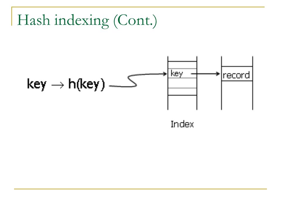
188. Hash based indexing Instead of keeping sequential indexes as in B-Tree the indexes are stored using hashes It is good for columns having exact number

189. Hash indexing (Cont.)

191. Example of B-Tree limitation

192. Conventional indexes disadvantages Conventional indexing comes in two types which includes, B-Tree and Hash indexing. There disadvantages are as follows It maps columns of tables into index but it does not provide any information about joining of this column with other tables Consumes a lot of memory when number of rows are too many These indexes are made for OLTP systems they do not take advantage of the stability of data in data warehouse for bulk updates

193. 193 Questions?

194. References [1] Abdullah, A.: “Data warehousing handouts”, Virtual University of Pakistan [2] Ricardo, C. M.: “Database Systems: Principles Design and Implementation”, Macmillan Coll Div. [3] Junk Dimension, http://www.1keydata.com/datawarehousing/junk- dimension.html http://www.1keydata.com/datawarehousing/junk- dimension.html [4] Advanced Topics of Dimensional Modeling https://mis.uhcl.edu/rob/Course/DW/Lectures/Advanced %20Dimensional%20Modeling.pdf https://mis.uhcl.edu/rob/Course/DW/Lectures/Advanced %20Dimensional%20Modeling.pdf [5] http://en.wikipedia.org/wiki/OLAP_cubehttp://en.wikipedia.org/wiki/OLAP_cube 194

195. References [6] http://www.mssqltips.com/sqlservertutorial/2011/processi ng-dimensions-and-cube/ http://www.mssqltips.com/sqlservertutorial/2011/processi ng-dimensions-and-cube/ [7] http://dev.mysql.com/doc/refman/5.1/en/partitioning- hash.html