Download presentation
Presentation is loading. Please wait.

1
Signal Analysis and Imaging Group Department of Physics University of Alberta
Regularized Migration/Inversion Henning Kuehl (Shell Canada) Mauricio Sacchi (Physics, UofA) Juefu Wang (Physics, UofA) Carrie Youzwishen (Exxon/Mobil) This doc -> Good afternoon everyone, I’m giving a talk on seismic wavefield reconstruction for AVA imaging .
 Mauricio Sacchi (Physics, UofA) Juefu Wang (Physics, UofA) Carrie Youzwishen (Exxon/Mobil) This doc -> Good afternoon everyone, I’m giving a talk on seismic wavefield reconstruction for AVA imaging .")
2
Outline Motivation and Goals
Migration/inversion - Evolution of ideas and concepts Quadratic versus non-quadratic regularization two examples The migration problem RLS migration with quadratic regularzation Examples RLS migration with non-quadratic regularization Summary

3
Motivation To go beyond the resolution provided by the data (aperture and band-width) by incorporating quadratic and non-quadratic regularization terms into migration/inversion algorithms This is not a new idea… The motivation we regularize seismic data before wave equation, without the regulariztion. AVA imaging may lack of amplidued fidelity due to uneven distrubution of offset in CDP bins. is AVA imaging, no matter ray tracing based Kirchhoff GRT, or wave equation based, they can have problem of lack of amplitude fidelity dues to uneven distribution of offset in CDP bins. And It’s often true for seismic data, especially in 3D. The problem oftenOne of the way to solve this problem is to use interpolation. In this talk, I will show you how interpolation of seismic data can be used to improve that we want to find a way to regularize seismic data before pre-stack 3D wave equation imaging. As we know that in 3D, AVA imaging is often lack of amplitude fidelity due to uneven distribution of offset in CDP bins
 by incorporating quadratic and non-quadratic regularization terms into migration/inversion algorithms. This is not a new idea… The motivation we regularize seismic data before wave equation, without the regulariztion. AVA imaging may lack of amplidued fidelity due to uneven distrubution of offset in CDP bins. is AVA imaging, no matter ray tracing based Kirchhoff GRT, or wave equation based, they can have problem of lack of amplitude fidelity dues to uneven distribution of offset in CDP bins. And It’s often true for seismic data, especially in 3D. The problem oftenOne of the way to solve this problem is to use interpolation. In this talk, I will show you how interpolation of seismic data can be used to improve that we want to find a way to regularize seismic data before pre-stack 3D wave equation imaging. As we know that in 3D, AVA imaging is often lack of amplitude fidelity due to uneven distribution of offset in CDP bins.")
4
Evolution of ideas and concepts
Migration with Adjoint Operators [Current technology] RLS Migration (Quadratic Regularization) [Not in production yet] RLS Migration (Non-Quadratic Regularization) [??] The motivation we regularize seismic data before wave equation, without the regulariztion. AVA imaging may lack of amplidued fidelity due to uneven distrubution of offset in CDP bins. is AVA imaging, no matter ray tracing based Kirchhoff GRT, or wave equation based, they can have problem of lack of amplitude fidelity dues to uneven distribution of offset in CDP bins. And It’s often true for seismic data, especially in 3D. The problem oftenOne of the way to solve this problem is to use interpolation. In this talk, I will show you how interpolation of seismic data can be used to improve that we want to find a way to regularize seismic data before pre-stack 3D wave equation imaging. As we know that in 3D, AVA imaging is often lack of amplitude fidelity due to uneven distribution of offset in CDP bins Resolution
 [Not in production yet] RLS Migration (Non-Quadratic Regularization) [ ] The motivation we regularize seismic data before wave equation, without the regulariztion. AVA imaging may lack of amplidued fidelity due to uneven distrubution of offset in CDP bins. is AVA imaging, no matter ray tracing based Kirchhoff GRT, or wave equation based, they can have problem of lack of amplitude fidelity dues to uneven distribution of offset in CDP bins. And It’s often true for seismic data, especially in 3D. The problem oftenOne of the way to solve this problem is to use interpolation. In this talk, I will show you how interpolation of seismic data can be used to improve that we want to find a way to regularize seismic data before pre-stack 3D wave equation imaging. As we know that in 3D, AVA imaging is often lack of amplitude fidelity due to uneven distribution of offset in CDP bins. Resolution.")
5
Evolution of ideas and concepts
Migration with Adjoint Operators 1 RLS Migration (Quadratic Regularization) 2 RLS Migration (Non-Quadratic Regularization) The motivation we regularize seismic data before wave equation, without the regulariztion. AVA imaging may lack of amplidued fidelity due to uneven distrubution of offset in CDP bins. is AVA imaging, no matter ray tracing based Kirchhoff GRT, or wave equation based, they can have problem of lack of amplitude fidelity dues to uneven distribution of offset in CDP bins. And It’s often true for seismic data, especially in 3D. The problem oftenOne of the way to solve this problem is to use interpolation. In this talk, I will show you how interpolation of seismic data can be used to improve that we want to find a way to regularize seismic data before pre-stack 3D wave equation imaging. As we know that in 3D, AVA imaging is often lack of amplitude fidelity due to uneven distribution of offset in CDP bins Resolution
 2 RLS Migration (Non-Quadratic Regularization) The motivation we regularize seismic data before wave equation, without the regulariztion. AVA imaging may lack of amplidued fidelity due to uneven distrubution of offset in CDP bins. is AVA imaging, no matter ray tracing based Kirchhoff GRT, or wave equation based, they can have problem of lack of amplitude fidelity dues to uneven distribution of offset in CDP bins. And It’s often true for seismic data, especially in 3D. The problem oftenOne of the way to solve this problem is to use interpolation. In this talk, I will show you how interpolation of seismic data can be used to improve that we want to find a way to regularize seismic data before pre-stack 3D wave equation imaging. As we know that in 3D, AVA imaging is often lack of amplitude fidelity due to uneven distribution of offset in CDP bins. Resolution.")
6
Evolution of ideas and concepts
Two examples LS Deconvolution Sparse Spike Deconvolution LS Radon Transforms HR Radon Transforms The motivation we regularize seismic data before wave equation, without the regulariztion. AVA imaging may lack of amplidued fidelity due to uneven distrubution of offset in CDP bins. is AVA imaging, no matter ray tracing based Kirchhoff GRT, or wave equation based, they can have problem of lack of amplitude fidelity dues to uneven distribution of offset in CDP bins. And It’s often true for seismic data, especially in 3D. The problem oftenOne of the way to solve this problem is to use interpolation. In this talk, I will show you how interpolation of seismic data can be used to improve that we want to find a way to regularize seismic data before pre-stack 3D wave equation imaging. As we know that in 3D, AVA imaging is often lack of amplitude fidelity due to uneven distribution of offset in CDP bins Quadratic Regularization Stable and Fast Algorithms Low Resolution Non-quadratic Regularization Requires Sophisticated Optimization Enhanced Resolution

7
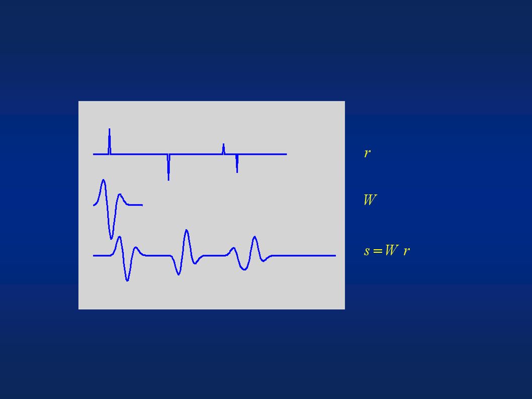
Deconvolution Quadratic versus non-quadratic regularization

8
Convolution / Cross-correlation / Deconv
Deconvolution Here is a toy example of the linear equation, Assume complete data consists of M=5 consecutive samples x1 x2 …, a sampling set N indicates the position of Known sample are at 2 3 5, so the incomplete data y consists of x(2) x(3) x(5). The sampling opertor is a 0/1 matrix. It is obvious that The linear systerm is underdetermined. we have more unknowns than observation. The solutions to such a system is non-unique. In general, we solve this type of problem by restricting the class of solution by providing suitable prior information.
 x(3) x(5). The sampling opertor is a 0/1 matrix. It is obvious that The linear systerm is underdetermined. we have more unknowns than observation. The solutions to such a system is non-unique. In general, we solve this type of problem by restricting the class of solution by providing suitable prior information.")
9
Quadratic and Non-quadratic Regularization
Cost Quadratic Here is a toy example of the linear equation, Assume complete data consists of M=5 consecutive samples x1 x2 …, a sampling set N indicates the position of Known sample are at 2 3 5, so the incomplete data y consists of x(2) x(3) x(5). The sampling opertor is a 0/1 matrix. It is obvious that The linear systerm is underdetermined. we have more unknowns than observation. The solutions to such a system is non-unique. In general, we solve this type of problem by restricting the class of solution by providing suitable prior information. Non-quadratic
 x(3) x(5). The sampling opertor is a 0/1 matrix. It is obvious that The linear systerm is underdetermined. we have more unknowns than observation. The solutions to such a system is non-unique. In general, we solve this type of problem by restricting the class of solution by providing suitable prior information. Non-quadratic.")
11
Adj LS HR

12
Radon Transform Quadratic versus non-quadratic regularization

13
LS Radon q h

14
HR Radon q h

15
Modeling / Migration / Inversion
De-blurring problem Here is a toy example of the linear equation, Assume complete data consists of M=5 consecutive samples x1 x2 …, a sampling set N indicates the position of Known sample are at 2 3 5, so the incomplete data y consists of x(2) x(3) x(5). The sampling opertor is a 0/1 matrix. It is obvious that The linear systerm is underdetermined. we have more unknowns than observation. The solutions to such a system is non-unique. In general, we solve this type of problem by restricting the class of solution by providing suitable prior information.
 x(3) x(5). The sampling opertor is a 0/1 matrix. It is obvious that The linear systerm is underdetermined. we have more unknowns than observation. The solutions to such a system is non-unique. In general, we solve this type of problem by restricting the class of solution by providing suitable prior information.")
16
Back to migration Inducing a sparse solution via non-quadratic regularization appears to be a good idea (at least for the two previous examples) Q. Is the same valid for Migration/Inversion?

17
Back to migration Inducing a sparse solution via non-quadratic regularization appears to be a good idea (at least for the two previous examples) Q. In the same valid for Migration/Inversion? A. Not so fast… First, we need to define what we are inverting for…

18
Migration as an inverse problem
Forward Adjoint Data “Image” or Angle Dependent Reflectivity

19
Migration as an inverse problem
There is No general agreement about what type of regularization should be used when inverting for m=m(x,z)… Geology is too complicated… For angle dependent images, m(x,z,p), we attempt to impose horizontal smoothness along the “redundant” variable in the CIGs: Kuehl, 2002, PhD Thesis UofA url: cm-gw.phys.ualberta.ca~/sacchi/saig/index.html
… Geology is too complicated… For angle dependent images, m(x,z,p), we attempt to impose horizontal smoothness along the redundant variable in the CIGs: Kuehl, 2002, PhD Thesis UofA. url: cm-gw.phys.ualberta.ca~/sacchi/saig/index.html.")
20
Quadratic Regularization Migration Algorithm Features:
DSR/AVP Forward/Adjoint Operator (Prucha et. al, 1999) PSPI/Split Step Optimization via PCG 2D/3D (Common Azimuth) MPI/Open MP Kuehl and Sacchi, Geophysics, January 03 [Amplitudes in 2D]
 PSPI/Split Step. Optimization via PCG. 2D/3D (Common Azimuth) MPI/Open MP. Kuehl and Sacchi, Geophysics, January 03 [Amplitudes in 2D]")
21
2D - Synthetic data example

22
Marmousi model (From H. Kuehl Thesis, UofA, 02)
AVA target Velocity Density

23
Migrated AVA CMP position [m] Ray parameter [mu s/m] 7000 7500 8000
200 400 600 800 0.5 0.5 1.0 1.0 ] ] m m k k [ [ h h t t p 1.5 p 1.5 e e D D 2.0 2.0 2.5 2.5
![Migrated AVA CMP position [m] Ray parameter [mu s/m]](http://slideplayer.com/slide/9489417/29/images/23/Migrated+AVA+CMP+position+%5Bm%5D+Ray+parameter+%5Bmu+s%2Fm%5D.jpg "] ] m. m. k. k. [ [ h. h. t. t. p p e. e. D. D")
24
Regularized Migrated AVA
p t h [ k m ] 0.5 1.0 1.5 2.0 2.5 7000 7500 8000 CMP position [m] 200 400 600 800 Ray parameter [mu s/m]

25
Migration RLSM 0.5 0.7 0.9 1.1 D e p t h [ k m ] 200 400 600 800
10 20 30 40 50 0.02 0.04 0.06 0.08 0.1 0.12 0.14 0.16 0.18 0.2 Angle of incidence (deg) Reflection coefficient 0.5 0.7 0.9 1.1 D e p t h [ k m ] 200 400 600 800 Ray parameter [mu s/m] Migration RLSM
![Migration RLSM D e p t h [ k m ]](http://slideplayer.com/slide/9489417/29/images/25/Migration+RLSM+D+e+p+t+h+%5B+k+m+%5D.jpg "Angle of incidence (deg) Reflection coefficient D. e. p. t. h. [ k. m. ] Ray parameter [mu s/m] Migration. RLSM.")
26
Incomplete CMP (30 %) Complete CMP 0.5 1.0 1.5 2.0 2.5 T i m e [ s c ]
0.5 1.0 1.5 2.0 2.5 T i m e [ s c ] 200 400 600 800 1000 1200 Offset [m] Complete CMP Incomplete CMP (30 %)
![Incomplete CMP (30 %) Complete CMP T i m e [ s c ]](http://slideplayer.com/slide/9489417/29/images/26/Incomplete+CMP+%2830+%25%29+Complete+CMP+T+i+m+e+%5B+s+c+%5D.jpg "T. i. m. e. [ s. c. ] Offset [m] Complete CMP. Incomplete CMP (30 %)")
27
Migration RLSM 0.5 0.7 0.9 1.1 D e p t h [ k m ] 200 400 600 800
200 400 600 800 Ray parameter [mu s/m] 10 20 30 40 50 0.02 0.04 0.06 0.08 0.1 0.12 0.14 0.16 0.18 0.2 Angle of incidence (deg) Reflection coefficient Migration RLSM
![Migration RLSM D e p t h [ k m ]](http://slideplayer.com/slide/9489417/29/images/27/Migration+RLSM+D+e+p+t+h+%5B+k+m+%5D.jpg "Ray parameter [mu s/m] Angle of incidence (deg) Reflection coefficient. Migration. RLSM.")
28
Constant ray parameter image (incomplete)
0.5 1.0 1.5 2.0 2.5 D e p t h [ k m ] 3000 4000 5000 6000 7000 8000 9000 CMP position [m] Constant ray parameter image (incomplete)
")
29
Constant ray parameter image (RLSM)
0.5 1.0 1.5 2.0 2.5 D e p t h [ k m ] 3000 4000 5000 6000 7000 8000 9000 CMP position [m] Constant ray parameter image (RLSM)
")
30
3D - Synthetic data example
(J Wang) Parameters for the 3D synthetic data x-CDPs : 40 Y-CDPs : 301 Nominal Offset: 50 dx=5 m dy=10 m dh=10 m 90% traces are randomly removed to simulate a sparse 3D data.
 Parameters for the 3D synthetic data. x-CDPs : 40. Y-CDPs : 301. Nominal Offset: 50. dx=5 m. dy=10 m. dh=10 m. 90% traces are randomly removed to simulate a sparse. 3D data.")
31
Incomplete Data Reconstructed data (after 12 Iterations)
4 adjacent CDPs Reconstructed data (after 12 Iterations)
")
32
A B C A: Iteration 1 B: Iteration 3 C: Iteration 12

33
At y=950 m, x=130 m

34
Misfit Curve Convergence – Misfit vs. CG iterations

35
Stacked images comparison (x-line 30)
A complete data B. Remove 90% traces C. least-squares

36
Field data example ERSKINE (WBC) orthogonal 3-D sparse land data set
dx=50.29m dy=33.5m Comment on Importance of W

37
CIG at x-line #10, in-line #71
Iteration 1 Iteration 3 Iteration 7 Cost Optimization

38
Stacked image, in-line #71
Migration RLS Migration

39
Stacked image, in-line #71
Migration RLS Migration

40
Image and Common Image Gather (detail)
")
41
Image and Common Image Gather (detail)
")
42
Stacked Image (x-line #10) comparison
Migration LS Migration

43
Non-quadratic regularization applied to imaging

44
Non-Quadratic Smoothing
Non-quadratic regularization But first, a little about smoothing: Quadratic Smoothing Non-Quadratic Smoothing

45
Quadratic regularization ->Linear filters
Non-quadratic -> Non-linear filters

46
Segmentation/Non-linear Smoothing

47
Segmentation/Non-linear Smoothing
1/Variance at edge position

48
2D Segmentation/Non-linear Smoothing

49
GRT Inversion - VSP (Carrie Youzwishen, MSc 2001)
* To test the algorithm, we use a 2D VSP model. An area 1 km square with a maximum acoustic potential of 1 is evaluated. The source and receiver geometry is shown on the first figure. The middle box is the synthetic (diffracted) data with a SNR of 5. The remaining figure shows the damped least squares solution.
 data with a SNR of 5. The remaining figure shows the damped least squares solution.")
50
Dx Dz m

51
HR Migration (Current Direction)
Quadratic constraint (Dp) to smooth along p (or h) Non-quadratic constraint to force vertical sparseness
 to smooth along p (or h) Non-quadratic constraint to force vertical sparseness.")
52
Example: we compare migrated images m(x,z,h) for the following 3 imaging methods:
Adj LS HR

53
Acoustic, Linearized, Constant V, Variable Density
Synthetic Model X(m) True Z(m) m(x,z) When the observations contain additive nosie rather than trying to fit exactly al observations, we attempt to fit the obsearvation in least squares sense. In this case we minimize a cost function that combins a data misfit function in conjuction with the model norm. Acoustic, Linearized, Constant V, Variable Density
 True. Z(m) m(x,z) When the observations contain additive nosie rather than trying to fit exactly al observations, we attempt to fit the obsearvation in least squares sense. In this case we minimize a cost function that combins a data misfit function in conjuction with the model norm. Acoustic, Linearized, Constant V, Variable Density.")
54
Pre-stack data d(s,g,t) Data
When the observations contain additive nosie rather than trying to fit exactly al observations, we attempt to fit the obsearvation in least squares sense. In this case we minimize a cost function that combins a data misfit function in conjuction with the model norm. Shots d(s,g,t)
")
55
Common offset images m(x,z,h) Adj Z(m)
CMP gather at 750m generated by a ray-tracing code. The code models (cylindrical) geometrical spreading but no transmission effects. The offset for the particular CMP ranges from 0m to 1280m. Middle: The same CMP after randomly removing of 90\% the data. Bottom: The reconstructed CMP using WMNI, the reconstructed offset ranges from 0m to 1200m. We first test our alogrithm on a simple, horizontally layered model. The horizontally layered model consists of four reflecting interfaces. The acoustic model parameters in terms of compressional velocities and densities range from 1900 m/s to 2500 m/s and from 1.6 g/$\textrm{cm}^3$ to 2.25 g/$\textrm{cm}^3$ , respectively. All interfaces are well separated. A ray tracing technique is used to generate the synthetic dataset. The ray-tracer takes advantage of the fact that, in a stratified medium, the ray parameter is constant for a particular ray. The geometrical spreading has been calculated assuming a cylindrical wavefront resulting in a $1 / \sqrt{r}$ amplitude scaling, where $r$ is the distance travelled by the ray. Notes that transmission losses is neglected in the synthetics. In Figure 1, top panel shows the CMP data at 750m. They exhibit a clear amplitude variation versus offset (AVO). the offsets range from 0 to 1295m incrementing by 20m. Figure 1 middle shows the same CMP after randomly removing $90$\% of the live traces. The incomplete CMPs (total 100) are used as the input for the reconstruction. We first perform Fourier transform along the time axis. Reconstructions are then carried at temporal frequencies along two spatial (CMP and offset) coordinates simultaneously. The output offset ranges 0m to 1200m for each CMP incrementing by 10m. Figure 1 bottom shows the reconstructed CMP at 750m using WMNI. m(x,z,h)
 geometrical spreading but no transmission effects. The offset for the. particular CMP ranges from 0m to 1280m. Middle: The same CMP. after randomly removing of 90\% the data. Bottom: The reconstructed CMP using WMNI, the reconstructed offset ranges from 0m to 1200m. We first test our alogrithm on a simple, horizontally layered model. The horizontally. layered model consists of four reflecting interfaces. The acoustic model. parameters in terms of compressional velocities and densities range from 1900 m/s to m/s and from 1.6 g/$\textrm{cm}^3$ to 2.25 g/$\textrm{cm}^3$ , respectively. All interfaces are well separated. A ray tracing technique is used to generate the synthetic dataset. The. ray-tracer takes advantage of the fact that, in a stratified medium, the ray parameter is. constant for a particular ray. The geometrical spreading has been calculated. assuming a. cylindrical wavefront resulting in a $1 / \sqrt{r}$ amplitude scaling, where $r$ is the distance. travelled by the ray. Notes that transmission losses is neglected in the synthetics. In Figure 1, top panel shows the CMP data at 750m. They exhibit a clear amplitude. variation versus offset (AVO). the offsets range from 0 to 1295m incrementing by 20m. Figure 1 middle shows the same CMP after randomly removing $90$\% of the live traces. The incomplete CMPs (total 100) are used as the input for the reconstruction. We first. perform Fourier transform along the time axis. Reconstructions are then carried at. temporal frequencies along two spatial (CMP and offset) coordinates simultaneously. The output offset ranges 0m to 1200m for each CMP incrementing by 10m. Figure 1 bottom shows the reconstructed CMP at 750m using WMNI. m(x,z,h)")
56
Common offset images LS Z(m) m(x,z,h)
 m(x,z,h)")
57
Common offset images HR Z(m) m(x,z,h)
 m(x,z,h)")
58
Stacked CIGs X(m) Adj Z(m) m(x,z)
 Adj Z(m) m(x,z)")
59
Stacked CIGs X(m) LS Z(m) m(x,z)
 LS Z(m) m(x,z)")
60
Stacked CIGs m(x,z) HR X(m) Z(m)
CMP gather at 750m generated by a ray-tracing code. The code models (cylindrical) geometrical spreading but no transmission effects. The offset for the particular CMP ranges from 0m to 1280m. Middle: The same CMP after randomly removing of 90\% the data. Bottom: The reconstructed CMP using WMNI, the reconstructed offset ranges from 0m to 1200m. We first test our alogrithm on a simple, horizontally layered model. The horizontally layered model consists of four reflecting interfaces. The acoustic model parameters in terms of compressional velocities and densities range from 1900 m/s to 2500 m/s and from 1.6 g/$\textrm{cm}^3$ to 2.25 g/$\textrm{cm}^3$ , respectively. All interfaces are well separated. A ray tracing technique is used to generate the synthetic dataset. The ray-tracer takes advantage of the fact that, in a stratified medium, the ray parameter is constant for a particular ray. The geometrical spreading has been calculated assuming a cylindrical wavefront resulting in a $1 / \sqrt{r}$ amplitude scaling, where $r$ is the distance travelled by the ray. Notes that transmission losses is neglected in the synthetics. In Figure 1, top panel shows the CMP data at 750m. They exhibit a clear amplitude variation versus offset (AVO). the offsets range from 0 to 1295m incrementing by 20m. Figure 1 middle shows the same CMP after randomly removing $90$\% of the live traces. The incomplete CMPs (total 100) are used as the input for the reconstruction. We first perform Fourier transform along the time axis. Reconstructions are then carried at temporal frequencies along two spatial (CMP and offset) coordinates simultaneously. The output offset ranges 0m to 1200m for each CMP incrementing by 10m. Figure 1 bottom shows the reconstructed CMP at 750m using WMNI.
 geometrical spreading but no transmission effects. The offset for the. particular CMP ranges from 0m to 1280m. Middle: The same CMP. after randomly removing of 90\% the data. Bottom: The reconstructed CMP using WMNI, the reconstructed offset ranges from 0m to 1200m. We first test our alogrithm on a simple, horizontally layered model. The horizontally. layered model consists of four reflecting interfaces. The acoustic model. parameters in terms of compressional velocities and densities range from 1900 m/s to m/s and from 1.6 g/$\textrm{cm}^3$ to 2.25 g/$\textrm{cm}^3$ , respectively. All interfaces are well separated. A ray tracing technique is used to generate the synthetic dataset. The. ray-tracer takes advantage of the fact that, in a stratified medium, the ray parameter is. constant for a particular ray. The geometrical spreading has been calculated. assuming a. cylindrical wavefront resulting in a $1 / \sqrt{r}$ amplitude scaling, where $r$ is the distance. travelled by the ray. Notes that transmission losses is neglected in the synthetics. In Figure 1, top panel shows the CMP data at 750m. They exhibit a clear amplitude. variation versus offset (AVO). the offsets range from 0 to 1295m incrementing by 20m. Figure 1 middle shows the same CMP after randomly removing $90$\% of the live traces. The incomplete CMPs (total 100) are used as the input for the reconstruction. We first. perform Fourier transform along the time axis. Reconstructions are then carried at. temporal frequencies along two spatial (CMP and offset) coordinates simultaneously. The output offset ranges 0m to 1200m for each CMP incrementing by 10m. Figure 1 bottom shows the reconstructed CMP at 750m using WMNI.")
61
CIGs CIG # CIG # CIG # 12 Adj LS Z(m) HR 0m Offset m

62
Data LS Prediction T(s) HR Prediction d(s,g,t) Shots
 HR Prediction d(s,g,t) Shots")
63
Conclusions Imaging/Inversion with the addition of quadratic and non-quadratic constraints could lead to a new class of imaging algorithms where the resolution of the inverted image can be enhanced beyond the limits imposed by the data (aperture and band-width). This is not a completely new idea. Exploration geophysicists have been using similar concepts to invert post-stack data (sparse spike inversion) and to design Radon operators. Finally, it is important to stress that any regularization strategy capable of enhancing the resolution of seismic images must be applied in the CIG domain. Continuity along the CIG horizontal variable (offset, angle, ray parameter) in conjunction with sparseness in depth, appears to be reasonable choice.
. This is not a completely new idea. Exploration geophysicists have been using similar concepts to invert post-stack data (sparse spike inversion) and to design Radon operators. Finally, it is important to stress that any regularization strategy capable of enhancing the resolution of seismic images must be applied in the CIG domain. Continuity along the CIG horizontal variable (offset, angle, ray parameter) in conjunction with sparseness in depth, appears to be reasonable choice.")
64
Acknowledgments EnCana Geo-X Veritas Schlumberger foundation NSERC
AERI 3D Real data set was provided by Dr Cheadle

Similar presentations
 domain, pattern-based ground roll removal Morgan P. Brown* and Robert G. Clapp Stanford Exploration Project Stanford University.>")


 Data The UBC Geophysical Inversion Facility Elliot Holtham and Douglas Oldenburg.>")


