Download presentation
Presentation is loading. Please wait.

1
Basic Detector Measurements: Photon Transfer Curve, Read Noise, Dark Current, Intrapixel Capacitance, Nonlinearity, Reference Pixels MR – May 19, 2014

2
Basic Detector Measurements: Photon Transfer Curve, Read Noise, Dark Current, Interpixel Capacitance, Nonlinearity, Reference Pixels MR – May 19, 2014

3
Mean-Variance aka Photon-Transfer Curve aka Shot-noise Method

4
Readout chain PN junction: QE Unit Cell: Cnode Pre-amplifier ADC photons electrons milliVolts Volts COUNTS 100,000 photons 80,000 electrons -200 mV 7.5 Volts 48,000 ADU detector

5
Signal falling on a pixel where associated noise

6
Gain conversion Passing the photogenerated signal thru a linear system with gain “g” [ADU/e]
![Gain conversion Passing the photogenerated signal thru a linear system with gain g [ADU/e]](http://images.slideplayer.com/29/9427129/slides/slide_6.jpg "Gain conversion Passing the photogenerated signal thru a linear system with gain g [ADU/e]")
7
Mean-Variance Relation The Variance in ADU is given by: and adding the readout noise:

8
RON adu 2 g[adu/e] Fowler & Joice, SPIE 1235, 151 (1990)
![RON adu 2 g[adu/e] Fowler & Joice, SPIE 1235, 151 (1990)](http://images.slideplayer.com/29/9427129/slides/slide_8.jpg "RON adu 2 g[adu/e] Fowler & Joice, SPIE 1235, 151 (1990)")
9
PN junction: QE Unit Cell: Cnode Pre-amplifier ADC photons electrons milliVolts Volts COUNTS 100,000 photons 80,000 electrons -200 mV 7.5 Volts 48,000 ADU detector Vreset

10
We can write or (usual g[e/adu])) or (at the ADC input) or knowing the Source Follower + Pre-amplifier conversion factor G(V/mV): node capacitance C0
![We can write or (usual g[e/adu])) or (at the ADC input) or knowing the Source Follower + Pre-amplifier conversion factor G(V/mV): node capacitance C0](http://images.slideplayer.com/29/9427129/slides/slide_10.jpg "We can write or (usual g[e/adu])) or (at the ADC input) or knowing the Source Follower + Pre-amplifier conversion factor G(V/mV): node capacitance C0")
11
“I don’t understand how it didn’t work. The science seemed so solid…!” King Julian, Madagascar II

12
Node Capacitance depends on Bias Finger et al. 2007 See Regan and Bergeron 2012, JWST-STScI-002925

13
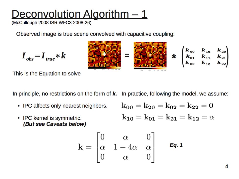
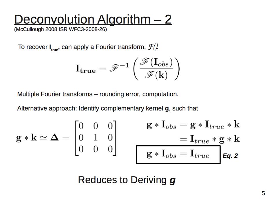
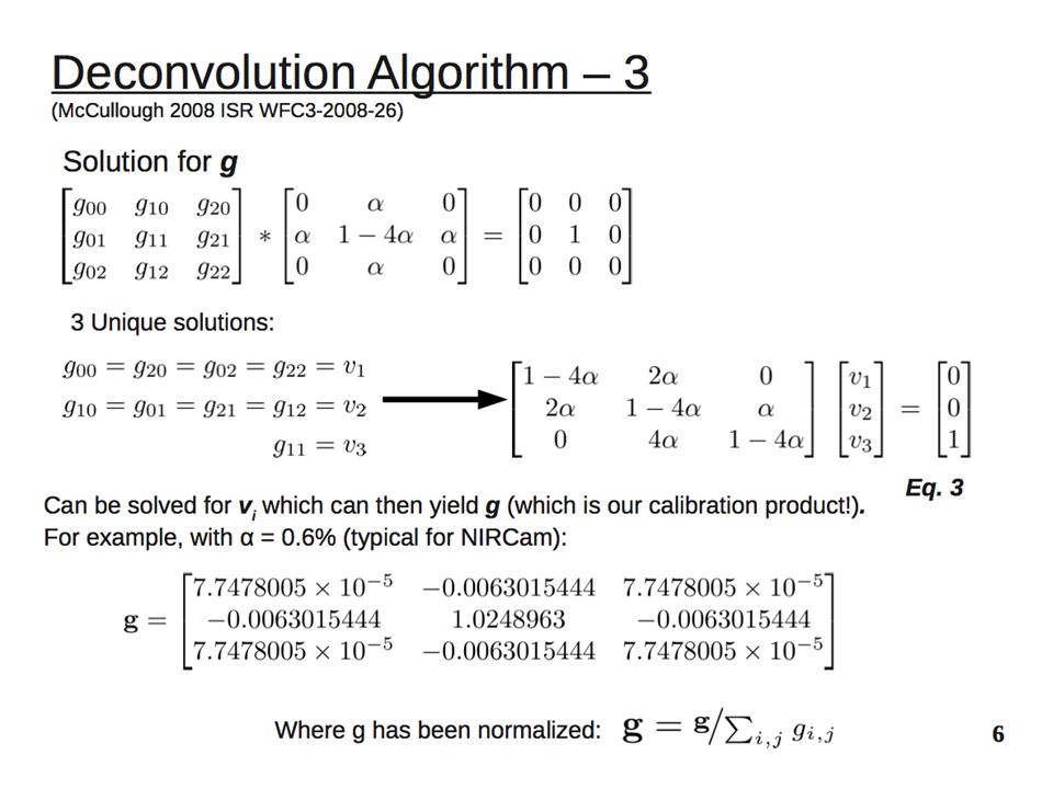
Interpixel coupling

14
In general, the variance is too low for any given signal. The capacitance is higher than C o ! INTERPIXEL CAPACITANCE PS this explains why they measured for years QE>100%!

15
What is Intrapixel Capacitance A capacitance requires an insulator between two conductors The depletion region is an insulator but the pixels are still shielded by the bulk n-material The space between the Indium Bump is an insulator between two pixels: capacitive coupling appears As a result, the charge seen by a pixel is spread to adjacent pixels With flat field illumination, the mean does not change but the variance decreases.

16
Effects Photometry is conserved: V 0 +4V i =V Image contrast is reduced (like “scattered light”) PSF/MTF is degraded
 PSF/MTF is degraded")
20
Readout Noise From Schubnell et al. Near Infrared Detectors for SNAP

21
Non linearity

22
IR detectors are non linear

23
Linearity is assumed at the beginning of the ramp linear fit to the first 20 samples

24
The “true” slope depends on the range of the assumed linear regime

25
How we do it now In the case of NICMOS and WFC3, we apply the following correction F are the measured counts F c are the true counts. The calibration process assumes that they are known (fit to the first part of the ramp). Known both F’s, we derive the correction coefficients c 2, c 3 and c 4 used for general linearity correction.
. Known both F’s, we derive the correction coefficients c 2, c 3 and c 4 used for general linearity correction..")
26
Problems with this approach 1) We do not really know what is the real slope of the calibration frame, and our estimate depends on the samples we use. 2) Physically, one has a linear true flux which is converted in a non-linear measured count rate by the detector. This is not what we model! We modulate the observed data to get the real flux; instead, we should modulate the real flux to get the observed data.
 Physically, one has a linear true flux which is converted in a non-linear measured count rate by the detector. This is not what we model. We modulate the observed data to get the real flux; instead, we should modulate the real flux to get the observed data..")
27
Residuals

28
Let’s look at the equation Instead of We can try with the physically more correct expression: i.e. we modulate the real flux F c to get F, not viceversa

29
Linearity correction From the values of c 2, c 3, an c 3 one can derive F c by solving the equation: Need to use an iterative method:

30
Results i=0 1 2 4

31
Check: different flux rate Same “detector”, i.e. exponential non-linearity term

32
Correction: old vs. new method Old New

33
Reference pixel correction

35
Horizontal Reference Pixels

36
Reference pixel correction (my way) 1) Subtract from each pixel its ramp averaged value. Work with RESIDUALS

37
2) The slopes of the four sectors are calculated by linearly fitting all horizontal reference pixels (rows 0-3 and 2044 ‐ 2047) against the corresponding read time. a) Sector 2 and 4 are flipped to match the timing sequence of sectors 1 and 3, “left to right”; b) Only the horizontal reference pixels are used to derive the slope. Using also the vertical reference pixels for the two outer sectors would provide a more accurate estimate of their two slopes, unbiased by the local values of the high frequency noise in the 2ms read time of the 4 rows at the top and bottom of the frames; however, a biased estimate is preferable, as the slopes will be consistently biased in all sectors.
 Sector 2 and 4 are flipped to match the timing sequence of sectors 1 and 3, left to right ; b) Only the horizontal reference pixels are used to derive the slope. Using also the vertical reference pixels for the two outer sectors would provide a more accurate estimate of their two slopes, unbiased by the local values of the high frequency noise in the 2ms read time of the 4 rows at the top and bottom of the frames; however, a biased estimate is preferable, as the slopes will be consistently biased in all sectors..")
38
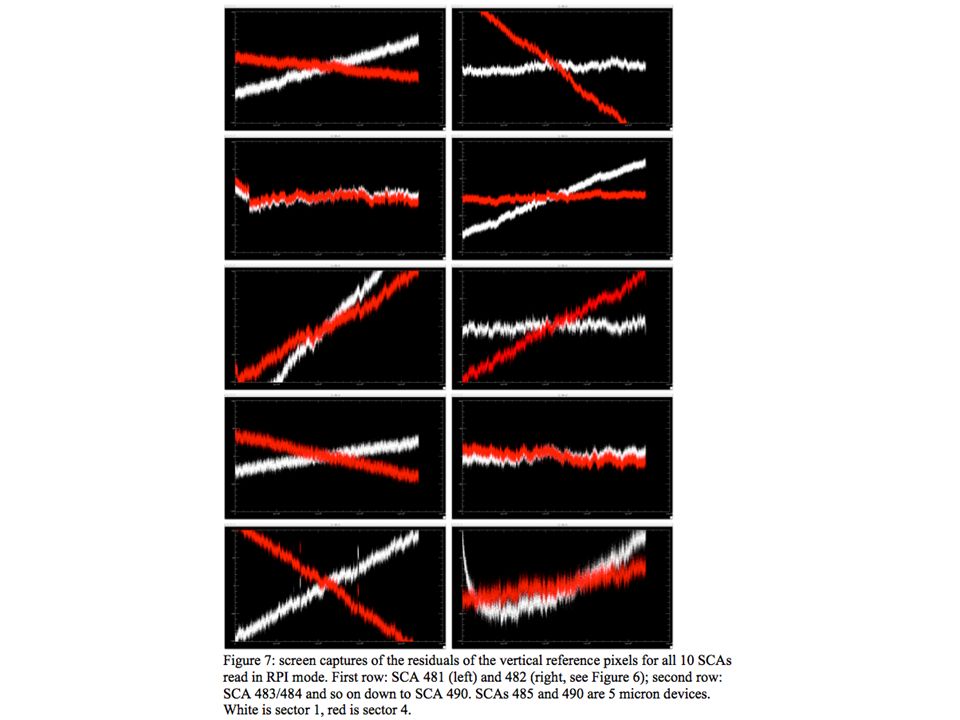
3) For each of the two outer sectors, the HIGH FREQUENCY noise is estimated by subtracting from the vertical reference pixels the appropriate value of the drift. a) For each sector, the noise is a vector of 2048 elements, one per row; b) The vertical reference pixels are first averaged row ‐ by ‐ row; for the 4+4 rows at the bottom and top one averages 512 pixels, for the other 2040 rows only 4 pixels are averaged; c) The time (needed to determine the drift term) is averaged in the same way;
 For each sector, the noise is a vector of 2048 elements, one per row; b) The vertical reference pixels are first averaged row ‐ by ‐ row; for the 4+4 rows at the bottom and top one averages 512 pixels, for the other 2040 rows only 4 pixels are averaged; c) The time (needed to determine the drift term) is averaged in the same way;.")
39
4) The noise vectors derived from the two outer sectors are averaged together to create the final noise model of the frame. At this point, it is possible to filter out the noise model to mitigate the uncertainties related to the average over only 8 horizontal reference pixels. Several strategies are possible.

40
Noise spectrum

43
5) The noise model is added to the slopes to produce a drift+noise vector for each sector. 6) The drift+noise vectors are replicated 512 times to produce a corrector frame. 7) The corrector frame is subtracted from the frame.
 The drift+noise vectors are replicated 512 times to produce a corrector frame. 7) The corrector frame is subtracted from the frame..")
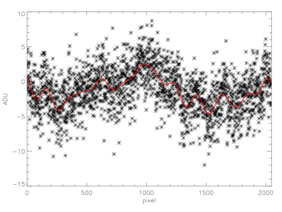
44
Without filter

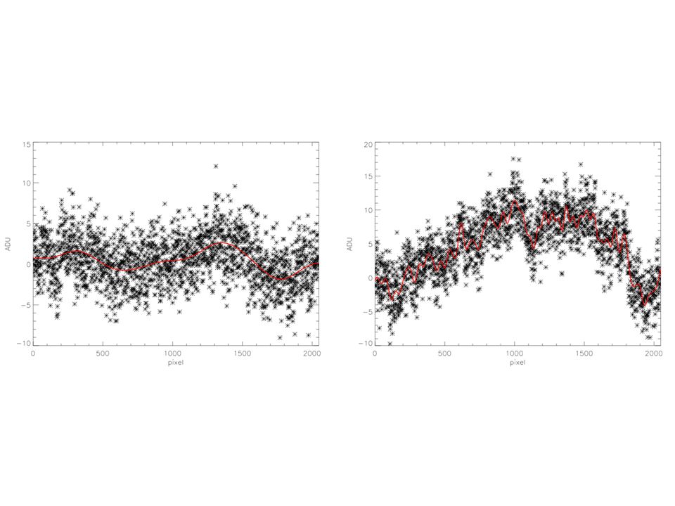
45
With filter

Similar presentations


>")


