1. Chapter 14: Inference for Regression

2. A brief review of chapter 4... (Regression Analysis: Exploring Association BetweenVariables )  Bi-variate data - relationships between 2 numeric, quantitative variables measured on same individual  Each individual appears as an point (x, y) on the scatter plot  Explanatory variable; response variable

3. Scatterplot; label & scale; look for overall patterns (DOFS)

4. Measuring Linear Association: Correlation or “r” Correlation (r) measures direction and strength of a linear relationship between two quantitative variables Correlation (r) is always between -1 and 1; makes no sense to have r = -13 or r = 27 Correlation (r) is not resistant (look at formula; based on mean) Correlation is for scatter plots (not LSRL) r is in standard units, so r doesn’t change if units are changed If we change from yards to feet, r is not effected

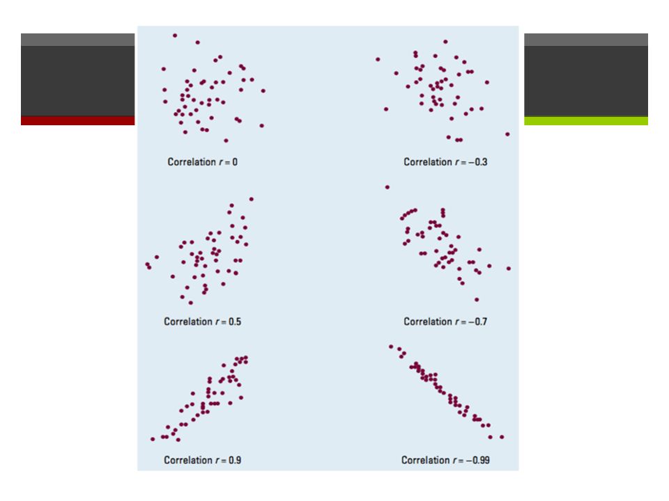
5. Measuring Linear Association: Correlation or “r”  r ≈0  not strong linear relationship  r close to 1  strong positive linear relationship  r close to -1  strong negative linear relationship

7. One better...Least Squares Regression Line (LSRL)

8. Least Squares Regression (predicts values)

9.  May be asked to interpret slope of LSRL & y-intercept, in context  Caution: Interpret slope of LSRL as the predicted or average change or expected change in the response variable given a unit change in the explanatory variable  NOT change in y for a unit change in x; LSRL is a model; models are not perfect

10. Extrapolation... What is it again??

11. Outliers & Influential Points  All influential points are outliers, but not all outliers are influential points. Influential points/observations: If removed would significantly change LSRL (slope and/or y-intercept)

12. Coefficient of Determination; r 2  r 2 tells us how well our LSRL describes our data; how well does this linear model fit the data  r 2 is always between 0 and 1 ; 0 ≤ r 2 ≤ 1  r 2, “fraction of the variation of the values of y that are explained by LSRL”  VERSUS r, correlation, -1 ≤ r ≤ 1; describes direction and strength of the linear relationship in a scatter plot

13. Chapter 14: Inference for Regression  We are now going to take all of that previous knowledge about bi-variate data and apply it to inference (forming judgments about population parameters on the basis of random sampling; a statistic)  Remember, = a + bx is just an estimate, a predictor, a statistic (like or ), based on a sample  Statistics vary from sample to sample

14. SRS BMW Cars (age & price)  What about another SRS of n = 7? Would data/points possibly be different?  So then would LSRL be different?  What about another SRS?  Data varies from sample to sample  Do we know the true population parameter? Do we have info on ALL BMW’s?

15. SRS BMW Cars (age & price)  So this LSRL is just based on THESE 7 pieces of data  We don’t know the true, unknown population parameter regression line, y = β o + β 1 x  But we can estimate the true, unknown regression line using a confidence interval... OR... we can test a claim using an hypothesis test

16. Let’s talk about conditions...  We need to be aware/check conditions before we perform inference (confidence intervals, hypothesis testing) with any situation (means, proportions, linear regression, one- sample, two-sample, Chi-Square, etc.)  If conditions are not met, our inference may be very inaccurate; worthless information

17. Conditions for Linear Regression Inference  1. Linearity: trend is linear (Use Residuals Plot to Check)  2. Normality: errors follow a Normal distribution with a mean of zero; N (0, σ ) (Use QQ Plot/Normal Probability Plot to Check)  3. Constant standard deviation: the standard deviation σ must be the same for all values of the predictor variable (Use Residuals Plot to Check)  4. Independence: Errors must be independent of one another (review raw data and collection process)

18. Residuals... we look at these to determine if conditions 1 & 3 are met  Least Squares Regression Line is not perfect, but it’s the best model we have  All points on the scatter plot don’t fit perfectly on the LSRL; very common  Vertical distances from point to LSRL are called “residuals,” or left-overs

19. Residuals: Observed y value – expected y value  LSRL is the line that creates the least “left-overs,” aka least residuals

20. Graphical Tool: Residuals Plot  We plot the residuals (left overs, points on scatterplot that are above or below LSRL) to determine if a line is the best model to describe our scatterplot of bivariate data  Perhaps a line isn’t the best model…. Maybe a quadratic curve or a log curve or square root function is a better model for the data

21. Residuals Plot (truck example)  On left is scatter plot & LSRL; on right is residuals plot

22. Graphical Tool: Residuals Plot  To check the linearity and the constant standard deviation conditions, should have no obvious pattern, random, unstructured  In the below case, both conditions are met

23. Residuals Plot  If there is an obvious pattern, conditions 1 & 3 are not met

24. Condition #2: Normality...  Errors must follow a Normal distribution  Can examine a Normal Probability Plot (NPP) (or a QQ Plot) of the residuals (left-overs)  If NPP is fairly linear, then condition #2 is satisfied

25. NPP that shows that errors do not follow a Normal distribution

26. Condition #4... Independence  Errors must be independent of one another  Exam the collection method of the data if possible  In most cases, we must assume independence until if/when we discover otherwise

27. Equation...for LSRL (sample statistic) Sample statistic: = a + b x where x is the value of the explanatory variable b is estimated slope (sample statistic) a is estimated y-intercept (sample statistic) is the estimated value of the response variable (sample statistic)

28. Equation... for true, unknown population parameter line Population parameter: y = β o + β 1 x x is the value of the explanatory variable β 1 is the true, actual (but unknown) population slope β 0 is the true, actual (but unknown) population y-intercept y is the true, actual (but unknown) value of the population parameter response variable

29. Hypothesis testing...  Majority of time, we are most interested in performing an hypothesis test on slope (not y-intercept) H o : Slope = 0 (OR β 1 = 0 OR there is no linear association between two variables OR correlation = 0) H a : Slope ≠ 0 (> or <) (OR β 1 ≠ 0 OR there is a linear association between the two variables OR correlation ≠ 0)... or > or <

30. Hypothesis testing...  Same 4 steps:  State null and alternative hypothesis  Check conditions  Do calculations  Interpret results in context

31. Random sample of 9 th grade students...... going on their annual backpacking trip each fall Is there a linear relationship between body weight and backpack weight? www.whfreeman.com/tps5e Body Weight (lbs) vs. Backpack Weight (lbs) Body Weight 120187109103131158116 Backpack Weight 26302624293128

32. H o : No linear relationship between body weight & backpack weight (or β 1 = 0) H a : There is a linear relationship between body weight & backpack weight (or β 1 ≠ 0) Conditions: Assume all conditions have been checked & met. Calculations: Enter data into Minitab (one column for body weight & another for backpack weight); then go to regression, simple regression. Careful of response & predictor (backwards). Choose linear, 95% confidence. Interpretation: Decision, α level, p-value, context. www.whfreeman.com/tps5e Body Weight (lbs) vs. Backpack Weight (lbs) Body Weight120187109103131158116 Backpack Weight26302624293128

33. Construct a confidence interval at the 95% level. Conditions: Assume all conditions have been checked & met. Calculations: Enter data into Minitab (one column for body weight & another for backpack weight); then go to regression, simple regression. Careful of response & predictor (backwards). Choose linear, 95% confidence. Interpretation: We are 95% confident that the true, unknown population parameter, the true slope, β, is between... www.whfreeman.com/tps5e Body Weight (lbs) vs. Backpack Weight (lbs) Body Weight120187109103131158116 Backpack Weight26302624293128

34. Do customers who stay longer at buffets give larger/smaller tips?  Xx Time (minutes)Tip ($) 235.00 392.75 447.75 555.00 617.00 658.88 679.01 705.00 747.29 857.5 906.00 996.50

35. Do customers who stay longer at buffets give larger/smaller tips?  A statistics student investigated this question as part of her project. She obtains a SRS of receipts which included this information.  Does this data provide convincing evidence that customers who stay longer tip differently than customers who stay shorter periods of time? H o : β = 0 (no relationship between variables) H a : β ≠ 0 (customers who stay longer give larger tips)  www.whfreeman.com/tps5e

36. Do customers who stay longer at buffets give larger/smaller tips? H o : β = 0 (no relationship between variables) H a : β ≠ 0 (customers who stay longer give larger tips) Conditions: Assume all conditions have been checked and met. Calculations: Enter data into Minitab and run calculations. Interpretation: Decision, α level, p-value, context. www.whfreeman.com/tps5e

37. Homework...  Homework  Section Quiz  Our next test...