1. Chapter 6: Agricultural Production Economics Production with One Input and One Output

2. A Production Function: Transformation of input into output A technical relationship (not behavioral)

3. Output: Corn Tobacco Wheat Beef Milk

4. Input: Seed Fertilizer Feed Machinery FERTILIZER 11-48-0 P205 N K20 JOHN DEERE

5. Fixed versus Variable Inputs Fixed-- Farmer does not expect to vary Over the planning horizon Variable-- Farmer expects to vary Over the planning horizon ? ? ? ? ? ?

6. Length of Planning Horizon: in the mind of the farmer 6 months? The Growing Season? 2 years? 10 years (for Christmas trees)? Only the farmer knows for sure 6 months ? 2 years ? 50 years ?

7. Old idea-- Inputs could be categorized Land--fixed Labor--variable Machinery--fixed (sort of!) Not a correct idea JOHN DEERE

8. Correct idea: Planning horizon determines whether inputs Short Run--All inputs fixed Intermediate Run--Some fixed, some variable Long Run--All inputs variable are fixed or variable

9. Inputs: Traditional list Land Labor Capital Management

10. With capital you can purchase land and labor Is management an input??

11. A Production Function: Y = f(X) Y = output such as bu. of corn X = input such as fertilizer f(x) = rule for transforming X into Y such as: Y = 3X Y = X Y =.3X +.05X -.002X Each of these are production functions 0.5 2 3

12. Y = f(X | X X X ) The Variable input The output Inputs treated as fixed Y X | X X X 3 Y or TPP TPP = Total Physical Product 1 2 3 4

13. Y X | X X X Y or TPP Y' Y'' Y''' X' X''X''' Specific amount of output from a specific amount of input 1 2 3 4 1 1 1

14. Marginal Product The incremental change in output associated with a 1 unit change in the use of the input

15. Marginal Product of input x: x = change in x y = change in y x = change in x = Marginal Product Also called Marginal Physical Product or MPP for short

16. Diminishing, Constant and Increasing Marginal Product

17. Constant Marginal Product Case 1:

18. Output Input (x) 0 1 2 3 4 2 4 6 8 (y) Constant slope y Constant Marginal Product

19. Output Input (x) 1 2 3 4 2 4 6 8 (y) 0 Constant slope y Triangles all the same size and slope = 2x 2 1 1 unit across 2 units up 2 2 2 1 1 1 Constant Marginal Product

20. Output Input (x) 1 2 3 4 2 4 6 8 (y) 0 Constant slope y = 2x 2 1 2 2 2 1 1 1 Each additional unit of X produces two additional units of Y Constant Marginal Product

21. Input (x) 1 2 3 4 Constant Marginal Product of b Output (y) 0 Constant slope of b y 1 1 1 1 b b b b b b b b =bx Each additional unit of x additional Units of y produces b The Marginal Product of an additional unit of x is b

22. Constant Marginal Product x x y y y/ x MPP

23. Constant Marginal Product x x y y 0 1 2 2 4 4 8 5 10 3 6 y / x MPP

24. Constant Marginal Product x x y y 0 1 2 2 4 4 8 5 10 3 6 1 1 1 1 1 y / MPP x

25. Constant Marginal Product x x y y 0 1 2 2 4 4 8 5 10 3 6 1 1 1 1 1 Y / MPP 2 2 2 2 2 x

26. Constant Marginal Product x x y y 0 1 2 2 4 4 8 5 10 3 6 1 1 1 1 1 Y / MPP 2 2 2 2 2 2/1 MPP = 2 everywhere x

27. Constant MPP x y = b x y b y = bx b = Marginal Product of an Additional Unit of x

28. Marginal Product Case 2: Increasing

29. Output (y) Input (x) 0 1 2 3 4 5 0.7 2 3.5 0.7 1.3 4.5 Increasing marginal returns to the variable input Increasing Marginal Product 3 6.5 11 1.5

30. x x y y 0 Y / x MPP 1 0.7 2 2.0 3 3.5 4 6.5 Increasing Marginal Product 5 11.0

31. x x y y 0 1 1 1 1 1 Y / x MPP 1 0.7 2 2.0 3 3.5 4 6.5 Increasing Marginal Product 5 11.0

32. x x y y 0 1 1 1 1 1 Y / x MPP.7 1.3 1.5 3. 4.5 1 0.7 2 2.0 3 3.5 4 6.5 Increasing Marginal Product 5 MPP increases as x increases 11.0

33. x x y y 0 1 1 1 1 1 Y / x MPP.7 1.3 1.5 3. 4.5 1 0.7 2 2.0 3 3.5 4 6.5.7/1 1.3/1 1.5/1 3.0/1 4.5/1 Increasing Marginal Product 5 MPP increases as x increases 11.0

34. Case 3: Decreasing (Diminishing) Marginal Product

35. Output (y) Input (x) 0 1 2 3 4 5 y = f(x) 5 2 1.5.3 1 1 1 1 1 5 7 8 8.5 8.8 Slope increases but at a decreasing rate Additional units of x produce less and less additional y Decreasing (Diminishing) Marginal Product

36. x x y y y / x MPP Decreasing Marginal Product

37. x x y y y / x MPP 0 1 5 2 7 3 8 4 8.5 5 8.8 Decreasing Marginal Product

38. x x y y y / x MPP 0 1 5 2 7 3 8 4 8.5 5 8.8 1 1 1 1 1 Decreasing Marginal Product

39. x x y y y / x MPP 0 1 5 2 7 3 8 4 8.5 5 8.8 1 1 1 1 1 5 2 1 0.5 Decreasing Marginal Product 0.3

40. x x y y y / x MPP 0 1 5 2 7 3 8 4 8.5 5 8.8 1 1 1 1 1 5 2 1 0.5 5/1 2/1 1/1.5/1.3/1 Decreasing Marginal Product As the use of x increases, MPP decreases 0.3

41. A Neoclassical Production Function X | X X X X 1 2 3 4 5

42. A Neoclassical Production Function Y X | X X X X 1 2 3 4 5

43. A Neoclassical Production Function Y Increasing MPP (and TPP) X | X X X X 1 2 3 4 5

44. A Neoclassical Production Function Y Increasing MPP (and TPP) Inflection Point X | X X X X 1 2 3 4 5

45. A Neoclassical Production Function Y Increasing MPP (and TPP) Inflection Point Decreasing MPP Increasing TPP X | X X X X 1 2 3 4 5

46. A Neoclassical Production Function Y Increasing MPP (and TPP) Inflection Point Decreasing MPP Increasing TPP Maximum TPP 0 MPP X | X X X X 1 2 3 4 5

47. A Neoclassical Production Function Y Increasing MPP (and TPP) Inflection Point Decreasing MPP Increasing TPP Maximum TPP 0 MPP Negative MPP Declining TPP X | X X X X 1 2 3 4 5

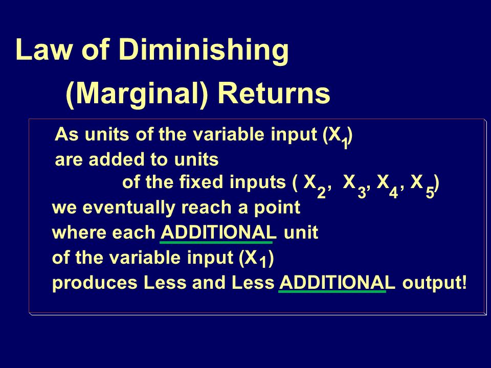
48. Law of Diminishing (Marginal) Returns As units of the variable input (X ) are added to units of the fixed inputs ( X, X, X, X ) we eventually reach a point where each ADDITIONAL unit of the variable input (X ) produces Less and Less ADDITIONAL output! 1 2 3 4 5 1

49. Y Increasing MPP (and TPP) Inflection Point Decreasing MPP Increasing TPP Maximum TPP 0 MPP Negative MPP Declining TPP Law of Diminishing Returns holds Starting Here X | X X X X 1 2 3 4 5

50. Y Increasing MPP (and TPP) Inflection Point Decreasing MPP Increasing TPP Maximum TPP 0 MPP Negative MPP Declining TPP X | X X X X 1 2 3 4 5

51. Y Increasing MPP (and TPP) Inflection Point Decreasing MPP Increasing TPP Maximum TPP 0 MPP Negative MPP Declining TPP MPP 0 X | X X X X 1 2 3 4 5

52. Y Increasing MPP (and TPP) Inflection Point Decreasing MPP Increasing TPP Maximum TPP 0 MPP Negative MPP Declining TPP MPP 0 X | X X X X 1 2 3 4 5 MPP X | X X X X 1 2 3 4 5

53. Y Increasing MPP (and TPP) Inflection Point Decreasing MPP Increasing TPP Maximum TPP 0 MPP Negative MPP Declining TPP MPP 0 X | X X X X 1 2 3 4 5 MPP X | X X X X 1 2 3 4 5

54. Y Increasing MPP (and TPP) Inflection Point Decreasing MPP Increasing TPP Maximum TPP 0 MPP Negative MPP Declining TPP MPP 0 X | X X X X 1 2 3 4 5 MPP X | X X X X 1 2 3 4 5

55. Average Physical Product The ratio of output to variable input Y/X Y/X | X X X X Average product of ALL units of X used (not the incremental unit) 1 2 3 4 5

56. X Y Y/X 2 16 8 3 21 7 4 24 6 5 25 5 6 18 3 0 0 undefined 1 7 7 Input Output (TPP) APP TPP and APP

57. Y TPP APP Point Inflection X

58. Y Line out of Origin TPP APP Point Inflection X

59. Y Line out of Origin Point of Tangency TPP APP Point Inflection X

60. Y Maximum APP Line out of Origin Point of Tangency TPP APP Point Inflection X

61. Y Maximum APP Line out of Origin Point of Tangency TPP APP Point Inflection X

62. Y Line out of Origin Ratio Y/X = Slope of Line From Origin TPP APP APP = Y/X Y X X

63. Y APP MAXIMUM Inflection Point X X APP APP, MPP 0 APP: Never Negative

64. Y APP MAXIMUM Inflection Point MPP = 0 MPP MAXIMUM X X MPP=APP APP MPP APP, MPP 0

65. Do They have a Relationship??? MPP APP Marginal Physical Product Average Physical Product MPP XX APP

66. 0 X | X X X X 1 2 3 4 5 MPP, APP

67. 0 X | X X X X 1 2 3 4 5 and Increasng APP Positive APP MPP, APP

68. 0 X | X X X X 1 2 3 4 5 and Increasng APP Positive MPP, APP Maximum APP

69. 0 X | X X X X 1 2 3 4 5 and Increasng APP Positive but Decreasing APP Positive Maximum APP MPP, APP

70. 0 X | X X X X 1 2 3 4 5 and Increasng APP Positive but Decreasing APP Positive Maximum APP MPP, APP

71. 0 X | X X X X 1 2 3 4 5 and Increasng APP Inflection Point of TPP Maximum MPP Positive but Decreasing APP Positive Maximum APP MPP, APP

72. 0 X | X X X X 1 2 3 4 5 Increasing MPP Decreasing MPP 0 MPP Maximum TPP Positive and Increasng APP Inflection Point of TPP Maximum MPP Positive but Positive but Decreasing APP Positive Maximum APP MPP=APP MPP, APP

73. MPP 0 X | X X X X 1 2 3 4 5 Increasing MPP Decreasing MPP 0 MPP Maximum TPP Positive Negative and Decreasing MPP and Increasng APP Inflection Point of TPP Maximum MPP Positive but Positive but Decreasing APP Positive Maximum APP MPP=APP MPP, APP

74. measures: responsiveness of output to changes in the use of Inputs Elasticity of Production A pure number (has no units)

75. Elasticity of Production % Change in output (Y) divided by % Change in input (X) % in output Y % in input X =

76. Elasticity of Production % in output Y % in input X Y/Y X/X = Y X X Y. MPP 1/APP = = MPP/APP

77. % in output Y % in input X = MPP/APP The Elasticity of Production (E p ) is the Ratio of MPP to APP

78. AVP E p = 0 $ MVP E p = 1 0 X | X X X X 1 2 3 4 5 E p > 1 (MPP>APP) 0<E p <1 E p < 0 Increasing MPP Decreasing MPP 0 MPP Maximum TPP Positive Negative and Decreasing MPP and Increasng APP

79. When the elasticity of production is greater than one, MPP lies above APP, APP is increasing, but MPP may be either increasing or decreasing. When the elasticity of production is between zero and 1, both MPP and APP are decreasing. However, MPP is positive here. Wnen the elasticity of production is negative, MPP is negative, and TPP is falling. However, APP still remains positive.

80. Profit Maximixation: and 1 output (Y) 1 input (X)

81. Assumptions: 1. Constant Input Price The producer can purchase as much or as little of the needed input at the going market price. No producer can affect input prices by the amount of the purchase.

82. 2. Constant Output Price No producer can affect the price of the output (Y) because of the individual production decision. The price of the input is V. The price of the output is P.

83. 3. Production Function Known with Certainty This is an unrealistic assumption for agriculture!

84. Profit = Total Revenue - Total Cost = TR - TC = PY –V X. but Y = f(X) so = Pf(X) – V X. Total Value of Product Total Factor Cost..

85. P f(X) - V X Total Value of Product Total Factor Cost Maximizing Profit: Maximize the difference between TVP and TFC TVP TFC..

86. What is the appearance of a TVP CURVE?

87. The TVP curve is a production function with the vertical axis measured in dollar value of output, not physical units TVP = P TPP. such as bushels or pounds.

88. TPP Y Production Function TPP P. $. =TVP TVP Curve X X TPP

89. What is the appearance of a Total Factor Cost (TFC) Curve?

90. Total Factor Cost (TFC) Curve TFC = V X TFC. $ V 1 x

91. TFC = V X TFC TVP TPP and TVP max. $ V 1 x Now Superimpose TVP Curve

92. TFC = V X TFC TVP Tangent TPP and TVP max. $ V 1 x

93. TFC = V X TFC TVP Tangent TPP and TVP max. $ V 1 x Right of APP max Left of TPP Max APP Max

94. TFC = V X TFC TVP Tangent TPP and TVP max. $ Maximum Vertical Distance = Maximum Profit Maximum Vertical Distance = Maximum Loss V 1 x

95. TFC = V X TFC 1 V TVP Tangent TPP max. $ Profit is maximum where slope of TVP = Slope of TFC X

96. Slope of TVP = Slope of TPP P. = MPP P. = MVP = Marginal Value of the Product So profits are maximum where: Slope of TVP = Slope of TFC MVP = MFC MVP = V MVP = the input price, assuming constant input and output prices

97. $ MVP 0 MVP= MPP P MFC = V Profit Max MVP=MFC=V Profit Min AVP=APP P TFC = V X TFC 1 V TVP Tangent TPP max. $ MVP=MFC=V AVP Max X X

98. Stages of Production

99. Stage I 0 units of X to level of X which Maximizes AVP

100. Stage II Level of X that Maximizes AVP to Level of X that Maximizes TPP (0 MVP and 0 MPP)

101. Stage III Level of X that Maximizes TPP (0 MPP) and Beyond...... Y Stage III X

102. The Rational Producer... 1. Never produces beyond the point of maximum TPP (input prices are never negative) 2. Produces at the point of maximum TPP only if the input is free! 3. Does not normally produce in stage I of Production Stage II is the Rational Stage of Production Where the profit maximizing point is found

103. $ AVP AVP=APP P. Why not stage I? Pick any point on the AVP curve. Draw an AVP curve. Average Value of the Product = Average Physical Product times the product price 0 X

104. $ AVP AVP=APP P. X' Area enclosed by rectangle is total revenue from the use of X' units of X X 0

105. $ X AVP=APP P. MVP = MPP P. Now add MVP curve Marginal Value Product = Marginal Physical Product times the product price 0

106. $ MVP Maximum Profit Total Factor Cost of Input X at profit max Now add MFC curve (MFC = V) Marginal Factor Cost = the price (V) of the input (X) AVP=APP P 0 X MFC=V

107. $ AVP=APP P. MVP Maximum Profit Total Revenue from sale of the product using profit maximizing level of X MFC=V X 0

108. $ X AVP=APP P. MVP Maximum Profit Total Factor Cost of Input X at Profit Max Cost of X Revenue-Cost=Profit MFC=V 0

109. $ X MVP AVP But if MFC > Maximum AVP Costs > Revenue Lose money where MVP=MFC, and shut down instead! Revenue MFC= V 0

110. $ X MVP AVP Revenue Cost of X MFC= V 0

111. $ X MVP AVP Revenue MFC= V Revenue fails to cover costs resulting in a loss as indicated Revenue Loss 0

112. Stages of Production and Elasticities of Production Stage I Ep > 1 Stage II 0 <Ep < 1 Stage III Ep < 0 Rational Stage where 0 <Ep < 1

113. AVP E p = 0 Stage I Stage IIStage III $ MVP E p = 1 0 X | X X X X 1 2 3 4 5 E p > 1 (MPP>APP) 0<E p <1 E p < 0 Increasing MPP Decreasing MPP 0 MPP Maximum TPP Positive Negative and Decreasing MPP and Increasng APP

114. AVP E p = 0 Stage I Stage IIStage III Demand Curve for input X $ MVP E p = 1 0 X | X X X X 1 2 3 4 5 E p > 1 (MPP>APP) 0<E p <1 E p < 0

115. The Demand Curve for a Singe Input All Points of Intersection Between MFC and MVP that lie in Stage II of Production The Quantity of Input the Producer Would Use to Maximize Profits at Each Possible Input Price