1. Chapter 4 Continuous Models Introduction –Independent variables are chosen as continuous values Time t Distance x, ….. –Paradigm for state variables Change over infinite small interval Change rate, rate of change –Ordinary differential equation (ODE) First order, second-order, higher orders –System of ODEs –Partial differential equations

2. Malthus’s Model Thomas R. Malthus (1766-1834): Father of population model In 1798, ``An Essay on the Principle of population’’ Profoundly impact on evolution theory of Charles Darwin (1809-1882) ``Malthus's observation was that, unchecked by environmental or social constraints, it appeared that human populations doubled every twenty-five years, regardless of the initial population size. Said another way, he posited that populations increased by a fixed proportion over a given period of time and that, absent constraints, this proportion was not affected by the size of the population. ‘’

3. Malthus’s Model ``By way of example, according to Malthus, if a population of 100 individuals increased to a population 135 individuals over the course of, say, five years, then a population of 1000 individuals would increase to 1350 individuals over the same period of time. ‘’ Let –t: time –N(t): the number of population at time t Balance equation:

4. Malthus’s model Consider the time interval

5. Malthus’s model Malthus’s assumption: –Unlimited resource & no migration –Birth rate and death rate are both constants The equation

6. Malthus’s model Phenomena –Population `explosion’: ``story of Prof. Yanchu Ma’’ –Population distinction –No change World population

7. The logistic model Assumption: (Verhulst, 1836) –Limited resource, no migration & death rate is constant –Birth rate decreases with increasing population

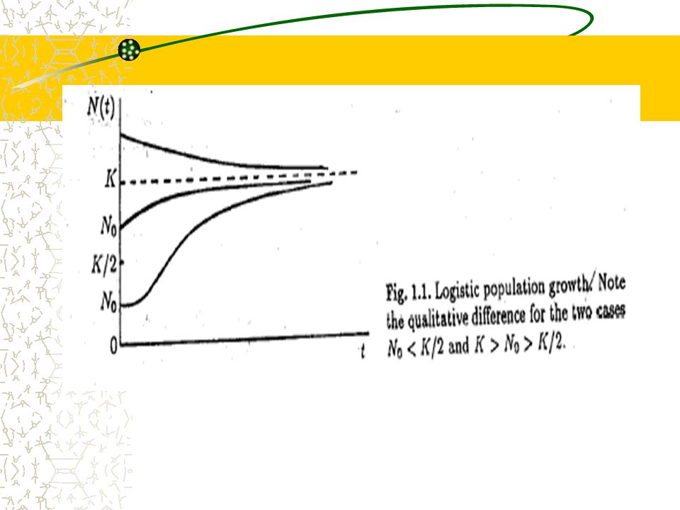
8. The logistic model The solution: Phenomena –Population distinction: –Equilibrium: Carrying capacity K: N(t) simply increase monotonically to K – Form a sigmoid character: slow-fast-slow change – fast-slow change N(t) decreases monotonically to K

10. Equilibrium & stability Consider autonomous ODE Equilibrium: Asymptotically stable: Conditions: –Stable: –Unstable:

11. Equilibrium & stability Reasons For Malthus’s model: N*=0 –Stable –Unstable For the logistic model: N*=0 or K –Stable: N*=K –Unstable: N*=0

12. Population with Harvesting Some examples –Population of Singapore or USA: immigration –Fish in a pound –Whale in the ocean Big environmental problems –Fishing grounds collapsed under over-fishing –Some animals are in danger of extinction due to indiscriminate hunting Big question: harvesting of renewable resources –Optimal harvest & without ruining the resource!!!!!

13. Harvest logistic model (I) Assumption: For fish, plants, etc –Limited resource & death rate is constant –Harvest depends linearly on the population –Birth rate decreases with increasing population

14. Harvest logistic model (I) We can find the solution, but here we are NOT so much interested in the value of N at a specific time instant t!! We are rather interested in –The terminal value of N when t goes to infinity?? ecologists who guard against extinction of animal or botanical species Scientists in agriculture who have to control pests Scientists in calculating fishing quotas, determine E!!! –Whether the population will die out in a finite period of time?? –Will N tend to a limit value when t goes to infinity?? –What is the optimal harvest strategy: Almost optimal harvest & the population can self renewable

15. Growth of f(N)

16. Harvest logistic model (I) The solution Phenomena –Equilibrium: –Yield or harvest is: –Maximum harvest:

17. Harvest logistic model (I) –Time scale of recovery after harvesting No harvest recovery time: With harvest & 0<E<r For fixed r, E increases, the recovery time increases Since the yield Y that is recorded, express T in the yield Y

18. Harvest logistic model (I) Optimal harvest strategy

19. Harvest logistic model (II) Assumption: –Limited resource & death rate is constant –Harvest fixed amount H per unit time –Birth rate decreases with increasing population –With

20. Harvest logistic model (II) We are rather interested in –The terminal value of N when t goes to infinity?? ecologists who guard against extinction of animal or botanical species Scientists in agriculture who have to control pests Scientists in calculating fishing quotas, scientist try to choose E in such a way that the annual catch is as large as possible without diminishing the stock (the maximum sustainable yield). Of course, the terminal value depends on E !!!

21. Harvest logistic model (II) Suppose the limit of N(t) exists, Plug into the equation It is equivalent Solution

22. Harvest logistic model (II) When, there exists a limit When, no limit!! –Population will extinct in a finite time T.

23. Harvest logistic model (II) F is a critical value in the sense that a harvesting rate which exceeds F must leads to the collapse of the stock Qualitative analysis: –Two different limiting values

24. Harvest logistic model (II) –Re-write the equation –Qualitative graph of the solution Case 1:, N(t) decreases near t=0 and remains decreasing as long as. Case 2: Case 3:, N(t) increases near t=0 and remains increasing as long as. Case 4: Case 5:, N(t) decreases near t=0. N(t) must be zero within a finite time T ( extinction time)

25. Harvest logistic model (II)

26. Example: The sandhill crane Grus canadensis in North American –It was protected since 1916 because it was on the endangered list –Repeated complaints of crop damage in USA and Canada led to hunting seasons since 1961. –These birds will not breed until they are 4 years old and normally will have a maximum life span of 25 years. –Two USA ecologists, R. Miller & D. Botkin studied it by constructing a simulation model with ten parameters to investigate the effect of different rates of hunting on the sandhill crane.

27. Harvest logistic model (II) –Use our logistic model II and their data, –Critical hunting rate is F=4800 birds per year –Take the initial value N(0)=194,600= which is the limit of the logistic model when E=0. –Comparison with Miller & Botkin Case 1: E>F

28. Harvest logistic model (II) Case 2: E<F –Our model is more optimistic than the prediction of Miller & Botkin, and surprisingly near to it!! Due to illegal hunters, Miller & Botkin plead for stricter control on indiscriminate hunting and for smaller quotas!!