1. Digital Image Processing
A wide variety of tools that we use to make remote sensing data provide even more information.
Tools include rectification, resampling, smoothing, edge enhancement, stretching etc.
The first tool considered is classification…

2. Classification Patterns in digital numbers = Patterns on the landscape
These tools use statistical analysis of multi-spectral images to enhance the information content provided by RS data.
Creating a thematic map

3. Multispectral image classification depends on the the fact that surface materials have different spectral reflectance patterns…. Different spectral signatures.

4. Supervised vs. Unsupervised
In ‘supervised’ classification the interpreter provides information about the classes he expects (or wants) to find.
“Training Sites” are selected on the image to identify the patterns in spectral space of classes/features that are to be identified
Unsupervised Classification… patterns inherent in the spectral data drive the classification process.

5. Unsupervised classification (contd.)
Unsupervised classification can often produce information that is not obvious to visual inspection.
Very useful for areas where ‘ground truth’ data is difficult to obtain
Purely spectral pattern recognition
The critical issue in ALL image classification is to equate ‘spectral class’ to ‘informational class’!!

6. “…The trick then becomes one of trying to relate the different clusters to meaningful ground categories. We do this by either being adequately familiar with the major classes expected in the scene, or, where feasible, by visiting the scene (ground truthing) and visually correlating map patterns to their ground counterparts…”

7. The process….
Step one: cluster analysis (Identifying clusters in the data)
Step two:Classification of pixels into classes based on cluster centers

8. Simple X Y example
(if it were only this simple in reality….)

9. A 3D version of spectral ‘clusters’… can easily be extended to n dimensional spectral space.

10. The clustering process
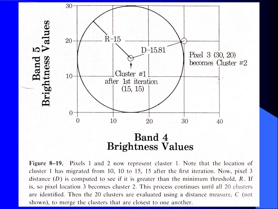
Virtually all programs use the identical algorithm “ISODATA”
Iterative Self-Organizing Data Analysis (ISODATA) Tou and Gonzalez 1974)
Begins by assigning class centriods in statistical space… (random assignment or some variation)

11. Cluster analysis….
The input parameters always requested by ISODATA include
The initial number of classes
A class separation distance (a lumping threshold)
And the number of iterations (or statistical threshold) that will define the end of the process

13. The first stage….cluster analysis
At the end of the first stage… nothing exists but a set of spectral coordinates in n dimensional space (where n is the number of spectral bands used in the classification)
Clusters have been defined based on the number of cluster centers you start with and the ‘lumping threshold’ which defines the distance between centers in spectral space
ERDAS reports this as a .sig file

15. The ‘right’ number of classes?
How does one select the ‘correct’ or ‘natural’ or ‘right’ number of classes?
The goal is INFORMATION CLASSES… not spectral classes…
“Expert Assessment and Visual Comparison” (it just looks better!)
Statistical tools?

16. Stage 2… putting all pixels into classes
There are three primary methods for assigning image pixels to classes
Minimum Distance to Means (mindist)
Parallellpiped
Maximum likelihood classification (maxlik)

17. The simplest classification… Minimum Distance to Means (MINDIST)
Pixels are assigned to a class based only on the minimum Euclidian distance to the closest cluster center….
Quick and easy but doesn’t consider variability in the data (the density of the cluster)

18. Parallepiped classification defines rectangular decision boundaries around classes…. The size of the rectangular decision boundary is defined by the variability in the spectral data….

19. Decision boundaries are defined by variability of the cluster in each dimension

20. Misidentified pixels…. A common problem

21. Maximum Likelihood Classification
This classification is very common
Used the variance and covariance of the data to define a ‘probability density function’ or probability surface….
(this assumes a ‘normal’ distribution of the data)

22. A probability density surface for the sample data set…
A probability density surface for the sample data set….. Based on the variability in the cluster, how likely is the inclusion of a given pixel

23. Probability contours for classes in 2 dimensional space… these statistical clouds extend in n dimensions….

24. Supervised Classification
Creating statistical clusters based on ‘a priori’ information
The interpreter knows what he wants to find… and creates ‘signature files’ (cluster centers) from ‘training sites’ on the image….

26. Choosing training sites…
Every class has to be fully identified

27. Training sites should be chosen from all across the image
Training sites should avoid edges where mixed pixels can add uncertainty to the classified image*
* A tool to accurately classify “mixed pixels” or highly heterogeneous areas is to choose training sites within the mixed area… the spectral signature for this class can be worked with independently.

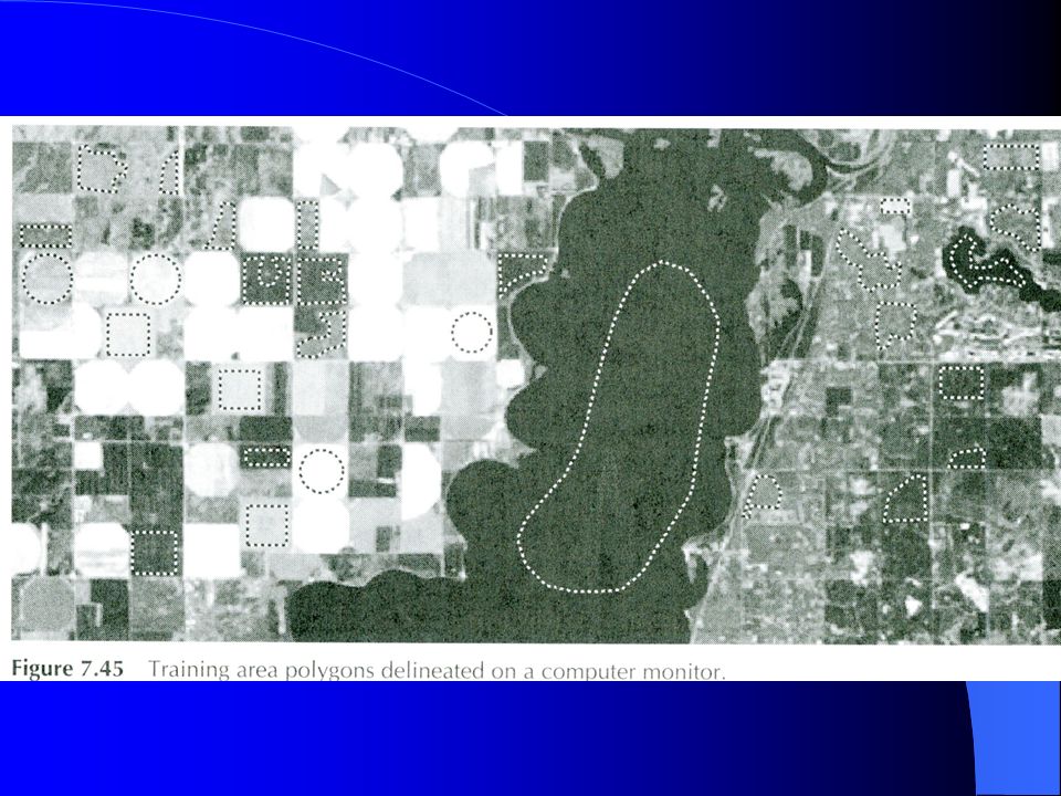
28. Training sites should include 10 to 100 times as many pixels as the total number of bands being used in the classification… e.g. for 7 TM bands training sites for each class ought to contain at least 70 – 700 pixels.
In agricultural applications not uncommon to have 100+ training sites / class
Polygons vs. “seeds”…. Rather than delineate the entire polygon, software can be used to ‘grow’ a training site…