Download presentation
Presentation is loading. Please wait.

1
Random Variables

2
A random variable X is a real valued function defined on the sample space, X : S R. The set { s S : X ( s ) [ a, b ] is an event}.
 [ a, b ] is an event}..")
3
Let S be the sample space of an experiment consisting of tossing two fair dice. Then, S = {(1, 1}, (1, 2),..., (6, 6)}. Let X be a random variable defined over S that assigns to each outcome the sum of the dice. Then, X ((1,1)) = 2, X ((1,2)) = 3,... X ((6,6)) = 12. Example 1
,..., (6, 6)}. Let X be a random variable defined over S that assigns to each outcome the sum of the dice. Then, X ((1,1)) = 2, X ((1,2)) = 3,... X ((6,6)) = 12. Example 1.")
4
Usually, we specify the distribution of a random variable without reference to the probability space.

5
If X denotes the random variable that is defined as the sum of two fair dice, then

6
If X denotes the random variable that is defined as the sum of two fair dice, then P { X = 2} = P {(1, 1)} = 1/36
} = 1/36")
7
If X denotes the random variable that is defined as the sum of two fair dice, then P { X = 2} = P {(1, 1)} = 1/36 P { X = 3} = P {(1, 2), (2, 1)} = 2/36
} = 1/36 P { X = 3} = P {(1, 2), (2, 1)} = 2/36")
8
If X denotes the random variable that is defined as the sum of two fair dice, then P { X = 2} = P {(1, 1)} = 1/36 P { X = 3} = P {(1, 2), (2, 1)} = 2/36 P { X = 4} = P {(1, 3), (3, 1), (2, 2)} = 3/36
} = 1/36 P { X = 3} = P {(1, 2), (2, 1)} = 2/36 P { X = 4} = P {(1, 3), (3, 1), (2, 2)} = 3/36")
9
If X denotes the random variable that is defined as the sum of two fair dice, then P { X = 2} = P {(1, 1)} = 1/36 P { X = 3} = P {(1, 2), (2, 1)} = 2/36 P { X = 4} = P {(1, 3), (3, 1), (2, 2)} = 3/36 P { X = 5} = P {(1, 4), (4, 1), (2, 3), (3, 2)} = 4/36
} = 1/36 P { X = 3} = P {(1, 2), (2, 1)} = 2/36 P { X = 4} = P {(1, 3), (3, 1), (2, 2)} = 3/36 P { X = 5} = P {(1, 4), (4, 1), (2, 3), (3, 2)} = 4/36")
10
If X denotes the random variable that is defined as the sum of two fair dice, then P { X = 2} = P {(1, 1)} = 1/36 P { X = 3} = P {(1, 2), (2, 1)} = 2/36 P { X = 4} = P {(1, 3), (3, 1), (2, 2)} = 3/36 P { X = 5} = P {(1, 4), (4, 1), (2, 3), (3, 2)} = 4/36 P { X = 6} = P {(1, 5), (5, 1), (2, 4), (4, 2), (3, 3)} = 5/36 P { X = 7} = P {(1, 6), (6, 1), (3, 4), (4, 3), (5, 2), (2, 5)} = 6/36 P { X = 8} = P {(2, 6), (6, 2), (3, 5), (5, 3), (4, 4)} = 5/36 P { X = 9} = P {(3, 6), (6, 3), (5, 4), (4, 5)} = 4/36 P { X = 10} = P {(4, 6), (6, 4), (5, 5)} = 3/36 P { X = 11} = P {(5, 6), (6, 5)} = 2/36 P { X = 12} = P {(6, 6)} = 1/36
} = 1/36 P { X = 3} = P {(1, 2), (2, 1)} = 2/36 P { X = 4} = P {(1, 3), (3, 1), (2, 2)} = 3/36 P { X = 5} = P {(1, 4), (4, 1), (2, 3), (3, 2)} = 4/36 P { X = 6} = P {(1, 5), (5, 1), (2, 4), (4, 2), (3, 3)} = 5/36 P { X = 7} = P {(1, 6), (6, 1), (3, 4), (4, 3), (5, 2), (2, 5)} = 6/36 P { X = 8} = P {(2, 6), (6, 2), (3, 5), (5, 3), (4, 4)} = 5/36 P { X = 9} = P {(3, 6), (6, 3), (5, 4), (4, 5)} = 4/36 P { X = 10} = P {(4, 6), (6, 4), (5, 5)} = 3/36 P { X = 11} = P {(5, 6), (6, 5)} = 2/36 P { X = 12} = P {(6, 6)} = 1/36")
11
The random variable X takes on values X = n, where n = 2,..., 12. Since the events corresponding to each value are mutually exclusive, then:

12
Let S be the sample space of an experiment consisting of tossing two fair coins. Then, S = {( H, H }, ( H, T ), ( T, H ), ( T, T )}. Let Y be a random variable defined over S that assigns to each outcome the number of heads Example 2
, ( T, H ), ( T, T )}. Let Y be a random variable defined over S that assigns to each outcome the number of heads Example 2.")
13
Let S be the sample space of an experiment consisting of tossing two fair coins. Then, S = {( H, H }, ( H, T ), ( T, H ), ( T, T )}. Let Y be a random variable defined over S that assigns to each outcome the number of heads. Then, Y is a random variable that takes on values 0, 1, 2: P ( Y =0) = 1/4 P ( Y =1) = 2/4 P ( Y =2) = 1/4. P ( Y =0) + P ( Y =1) + P ( Y =2) = 1. Example 2
, ( T, H ), ( T, T )}. Let Y be a random variable defined over S that assigns to each outcome the number of heads. Then, Y is a random variable that takes on values 0, 1, 2: P ( Y =0) = 1/4 P ( Y =1) = 2/4 P ( Y =2) = 1/4. P ( Y =0) + P ( Y =1) + P ( Y =2) = 1. Example 2.")
14
A die is repeatedly tossed until a six appears. Let X denote the number of tosses required, assuming successive tosses are independent. Example 3

15
A die is repeatedly tossed until a six appears. Let X denote the number of tosses required, assuming successive tosses are independent. The random variables X takes on values 1, 2,..., with respective probabilities: Example 3

16
A die is repeatedly tossed until a six appears. Let X denote the number of tosses required, assuming successive tosses are independent. The random variables X takes on values 1, 2,..., with respective probabilities: P ( X =1) = 1/6 P ( X =2) = (5/6)(1/6) P ( X =3) = (5/6) 2 (1/6) P ( X =4) = (5/6) 3 (1/6)... P ( X = n ) = (5/6) n -1 (1/6) Example 3
 = 1/6 P ( X =2) = (5/6)(1/6) P ( X =3) = (5/6) 2 (1/6) P ( X =4) = (5/6) 3 (1/6)... P ( X = n ) = (5/6) n -1 (1/6) Example 3.")
18
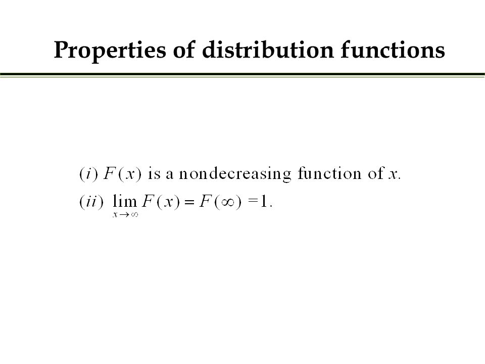
The distribution function F (also called cumulative distribution function (cdf)) of a random variable is defined by F ( x ) = P ( X ≤ x ), where x is a real number. Distribution functions

19
The distribution function F (also called cumulative distribution function (cdf)) of a random variable is defined by F ( x ) = P ( X ≤ x ), where x is a real number. Distribution functions upper case lower case

20
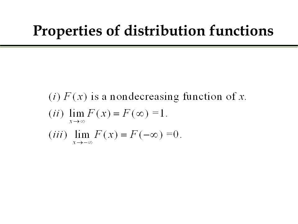
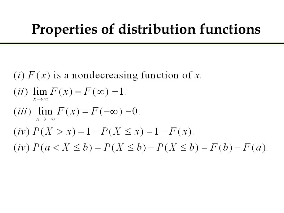
Properties of distribution functions

25
Note that P ( X < x ) does not necessarily equal F ( x ) since F ( x ) includes the probability that X equals x.
 does not necessarily equal F ( x ) since F ( x ) includes the probability that X equals x.")
26
A discrete random variable is a random variable that takes on either a finite or a countable number of states. Discrete random variables

27
The probability mass function (pmf) of a discrete random variable is defined by p ( x ) = P ( X = x ). If x takes on values x 1, x 2,..., then Probability mass function

28
The probability mass function (pmf) of a discrete random variable is defined by p ( x ) = P ( X = x ). If x takes on values x 1, x 2,..., then The cumulative distribution function F is given by Probability mass function

29
Let X be a random with pmf p (2) = 0.25, p (4) = 0.6, and p (6) = 0.15. Then, the cdf F of X is given by Example

30
Let X be a random with pmf p (2) = 0.25, p (4) = 0.6, and p (6) = 0.15. Then, the cdf F of X is given by Example

31
Let X be a random variable that takes on values 1 (success) or 0 (failure), then the pmf of X is given by p (0) = P ( X =0) = 1 - p and p (1) = P ( X =1) = p where 0 ≤ p ≤ 1 is the probability of “success.” A random variable that has the above pmf is said to be a Bernoulli random variable. The Bernoulli random variable

32
A random variable that has the following pmf is said to be a geometric random variable with parameter p. p ( n ) = P ( X = n ) = (1 – p) n -1 p, for n = 1, 2,.... The Geometric random variable
 = P ( X = n ) = (1 – p) n -1 p, for n = 1, 2,.... The Geometric random variable.")
33
A random variable that has the following pmf is said to be a geometric random variable with parameter p. p ( n ) = P ( X = n ) = (1 – p) n -1 p, for n = 1, 2,.... Example: A series of independent trials, each having a probability p of being a success, are performed until a success occurs. Let X be the number of trials required until the first success. The Geometric random variable
 = P ( X = n ) = (1 – p) n -1 p, for n = 1, 2,.... Example: A series of independent trials, each having a probability p of being a success, are performed until a success occurs. Let X be the number of trials required until the first success. The Geometric random variable.")
34
A random variable that has the following pmf is said to be a geometric random variable with parameters ( n, p ) The Binomial random variable
 The Binomial random variable")
35
Example: A series of n independent trials, each having a probability p of being a success and 1 – p of being a failure, are performed until a success occurs. Let X be the number of successes in the n trials.

36
A random variable that has the following pmf is said to be a Poisson random variable with parameter The Poisson random variable

37
The number of cars sold per day by a dealer is Poisson with parameter = 2. What is the probability of selling no cars today? What is the probability of receiving 100? Solution: P ( X =0) = e -2 0.135 P(X = 2)= e -2 (2 2 /2!) 0.270
 = e -2 P(X = 2)= e -2 (2 2 /2!) ")
38
Example: The number of cars sold per day by a dealer is Poisson with parameter = 2. What is the probability of selling no cars today? What is the probability of receiving 100? Solution: P ( X =0) = e -2 0.135 P(X = 2)= e -2 (2 2 /2!) 0.270
 = e -2 P(X = 2)= e -2 (2 2 /2!) ")
39
A continuous random variable is a random variable whose set of possible values is uncountable. In particular, we say that Continuous random variables

Similar presentations


 Random Variables and Distribution Functions.>")
, to each outcome ζ in the sample space of a random experiment. Domain.>")


