1. Ch4 Describing Relationships Between Variables

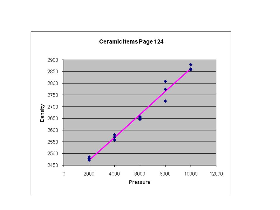
2. Section 4.1: Fitting a Line by Least Squares Often we want to fit a straight line to data. For example from an experiment we might have the following data showing the relationship of density of specimens made from a ceramic compound at different pressures. By fitting a line to the data we can predict what the average density would be for specimens made at any given pressure, even pressures we did not investigate experimentally.

4. For a straight line we assume a model which says that on average in the whole population of possible specimens the average density, y, value is related to pressure, x, by the equation The population (true) intercept and slope are represented by Greek symbols just like  and .

5. For the measured data we fit a straight line For the i th point, the fitted line or predicted value is The fitted line is most often determined by the method of “least squares”.

6. “Least squares” is the optimal method to use for fitting the line if – The relationship is in fact linear. – For a fixed value of x the resulting values of y are normally distributed with the same constant variance at all x values.

7. If these assumptions are not met, then we are not using the best tool for the job. For any statistical tool, know when that tool is the right one to use.

8. A least squares fit minimizes the sum of squared deviations from the fitted line minimize Deviations from the fitted line are called “residuals” We are minimizing the sum of squared residuals, called the “residual sum of squares.”

9. We need to minimize over all possible values of b 0 and b 1 a calculus problem.

10. The resulting formulas for the least squares estimates of the intercept and slope are

11. If, If we have average pressure, x, then we expect to get about average density, y.

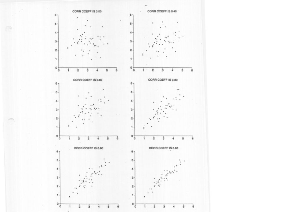
12. The sample (linear) correlation coefficient, r, is a measure of how “correlated” the x and y variable are. The correlation coefficient is between -1 and 1 +1 means perfectly positively correlated 0 means no correlation -1 means perfectly negatively correlated

13. The correlation coefficient is computed by

14. The slope, b 1, and the correlation coefficient are related by – is the standard deviation of y values and – is the standard deviation of x values. For every run on the x axis, the fitted line rises units on the y axis.

15. So if x is a certain number of standard deviations above average,, then y is, on average, the fraction r times that many standard deviations above average,..

16. For example if the correlation is r = 0.9 If the pressure, x, is 2 standard deviations above average Then we expect the density, y, will be about 0.9*(2) = 1.8 standard deviations above average.

19. lnterpretation of r 2 or R 2 R 2 = fraction of variation accounted for (explained) by the fitted line.

20. Pressurey = Densityy - mean(y-mean)^2 20002486-18132761 20002479-18835344 20002472-19538025 40002558-10911881 40002570-979409 40002580-877569 60002646-21441 60002657-10100 60002653-14196 80002724573249 8000277410711449 8000280814119881 10000286119437636 10000287921244944 10000285819136481 mean60002667sum0289366 st dev2927.7143.767 correlation0.991 correl^20.982

21. If we don't use the pressures to predict density – We use to predict every y i – Our sum of squared errors is = SS Total in Excel If we do use the pressures to predict density – We use to predict y i – = SS Residual in Excel

22. ObservationPredicted DensityResidualsResidual^2 12472.33313.667186.778 22472.3336.66744.444 32472.333-0.3330.111 42569.667-11.667136.111 52569.6670.3330.111 62569.66710.333106.778 72667.000-21.000441.000 82667.000-10.000100.000 92667.000-14.000196.000 102764.333-40.3331626.778 112764.3339.66793.444 122764.33343.6671906.778 132861.667-0.6670.444 142861.66717.333300.444 152861.667-3.66713.444 5152.666667sum

23. The percent reduction in our error sum of squares is Using x to predict y decreases the error sum of squares by 98.2%.

24. The reduction in error sum of squares from using x to predict y is – Sum of squares explained by the regression equation – 284,213.33 = SS Regression in Excel This is also the correlation squared. r 2 = 0.991 2 = 0.982

25. For a perfectly straight line All residuals are zero. – The line fits the points exactly. SS Residual = 0 SS Regression = SS Total – The regression equation explains all variation R 2 = 100% r = ±1 – r 2 = 1 If r=0, then there is no linear relationship between x and y R 2 = 0% Using x to predict y does not help at all.

26. Checking Model Adequacy With only single x variable, we can tell most of what we need from a plot with the fitted line.

27. Plotting residuals will be most crucial in section 4.2 with multiple x variables – But residual plots are still of use here. Plot residuals versus – Predicted values – Versus x – In run order – Versus other potentially influential variables, e.g. technician – Normal Plot of residuals

28. A residual plot gives us a magnified view of the increasing variance and curvature. This residual plot indicates 2 problems with this linear least squares fit The relationship is not linear – Indicated by the curvature in the residual plot The variance is not constant – So the least squares method isn't the best approach even if we handle the nonlinearity.

29. Don't fit a linear function to these data directly with least squares. With increasing variability, not all squared errors should count equally.

30. Some Study Questions What does it mean to say that a line fit to data is the "least squares" line? Where do the terms least and squares come from? We are fitting data with a straight line. What 3 assumptions (conditions) need to be true for a linear least squares fit to be the optimal way of fitting a line to the data? What does it mean if the correlation between x and y is -1? What is the residual sum of squares in this situation? If the correlation between x and y is 0, what is the regression sum of squares, SS Regression, in this situation? If x is 2 standard deviations above the average x value and the correlation between x and y is -0.6, the expected corresponding y values is how many standard deviations above or below the average y value?

31. Consider the following data. ANOVA dfSSMSFSignificance F Regression1124.0333124.0315.850.016383072 Residual431.37.825 Total5155.3333 Coefficients Standard Errort StatP-valueLower 95%Upper 95% Intercept-0.52.79732-0.17870.867-8.266605837.2666058 X1.5250.3830393.98130.0160.4615136982.5884863

32. What is the value of R 2 ? What is the least squares regression equation? How much does y increase on average if x is increased by 1.0? What is the sum of squared residuals? Do not compute the residuals; find the answer in the Excel output. What is the sum of squared deviations of y from y bar? By how much is the sum of squared errors reduced by using x to predict y compared to using only y bar to predict y? What is the residual for the point with x = 2?