1. Preferences vs constraints revisited Multilevel modelling of womens working time preferences in England and Scotland Pierre Walthery – CCSR – University of Manchester

2. Structure of the presentation Preferences, constraints, orientations to work: explaining womens labour force participation Reversing the perspective: modelling preferences Data & methods Main results Conclusions/future work

3. Women and the LM -- What A traditional pattern among British women: in, out, and in again -- maybe --later (Martin & Roberts 1984 Gustaffson et al ?). The cross-sectional view --mind the gaps: Activity Employment Earnings Gender segregation For a long time, a large number of empirical researchers seem to have stood somewhere in the middle in a tacit agreement.

4. Women and the LM Harmony was broken by Hakims presentation of her PT. She drew both on RCT and Revealed Preferences approaches. Contends that: Women can be divided into three broad work orientations based groups, the most important of which is made of adaptive women. Others are either work or family oriented. It is these lifestyle preferences, rather than social structure, or constraints that can best predict and explain womens subsequent labour market participation However, this is only true in countries where a real choice is possible: ie the US & the UK (as opposed to Sweden). P references, not attitudes are causal.

5. Gathered a large amount of reactions, most of which were quite critical. However: Had the merit to stimulate the discussion and subsequent research avenues; Put the issue of womens agency back at the centre of the academic debate (Walsh 2005). Alternative views: Classless women (Ginn et al 1996; McRae 2003) Polarization between women (Joshi et al; Crom p ton et al 1998 ) Preferences only loosely match behaviour, circularity (Crom p ton et al 2005). Preferences vary across time and following events in the lifecourse. Identities are ada ptable (Himmelweit & Sigala 2004) Mostly qualitative research has dealt with the contingency of p references Preferences and attitudes are for a large part dependent on a womans circumstances. Their relation to actual labour market is probably complex, time and path-dependent. Women and the labour market

6. Modelling preferences – in theory Semi freedom: social p ractice (Bourdieu) determined by a habitus within boundaries set by social structures. They could be seen as different interdependent layers of constraints and opportunities: The amount of economic, social, cultural capital women possess Gender structures -- ie gender roles / gender regimes (Connell) Institutions: labour market, childcare markets and facilities Cultural dimension (Duncan/Pffau-Effinger) Within these constraints, preferences are forming and evolving

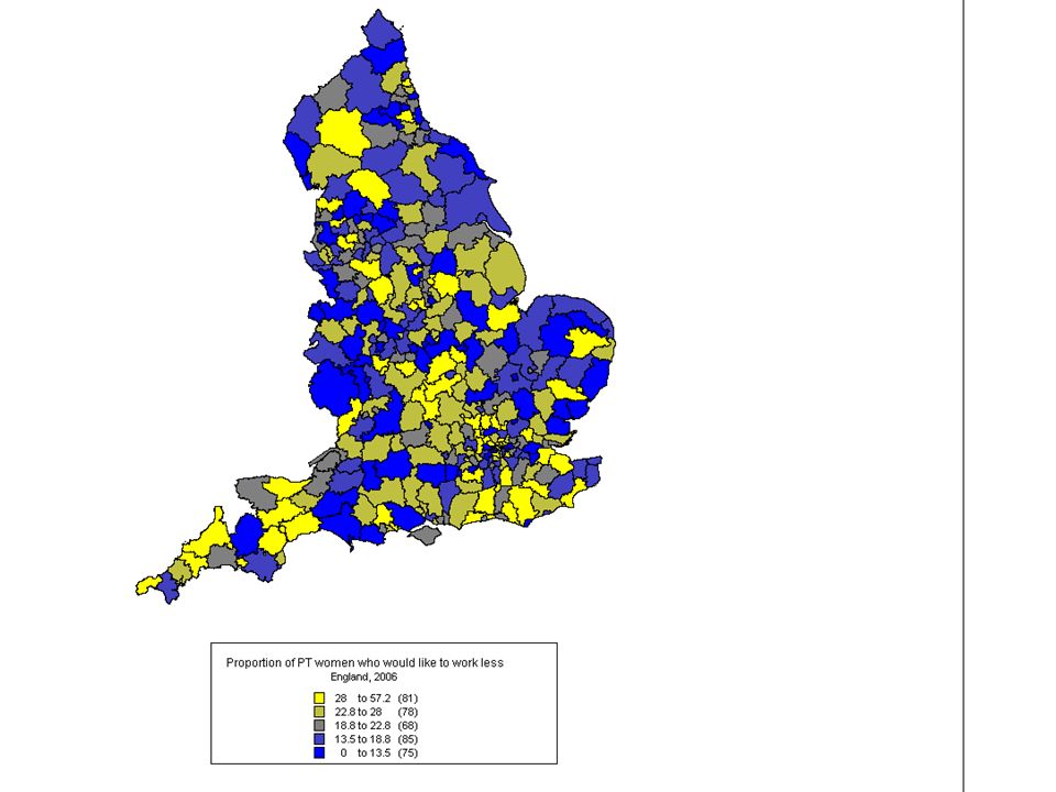
7. Modelling preferences – in practice Creating a statistical model accounting for variations in preferences: 1. Characteristics that are measurable at the individual level: Are individual/household circumstances, significantly associated to preferences? 2. Geography: Is there additional local-authority (LAD) based variation in preferences? Does this match any measured characteristics of the LAD (ie unemployment level, availability of childcare)? 3. Time. Not there yet. Working-time preferences as an indicator of willingness to get involved more/less in the labour market.

8. Data Special License Annual Population Survey for England and Scotland. Two quarters of the Labour Force Survey + booster samples Large scale stratified random sample (n>350,000): good geographical coverage, more reliable estimates Special licence APS provides information about LAD. Mostly hard data, very few questions about attitudes and preferences, orientations Do not allow easily allow to mix individual and household level variables Merged with: LAD- level reliable estimates from the 2001 Sample of Anonymised Records from the Census (Sars) Administrative records from Ofsted (2006) & the Scottish Executive (2006) about childcare places Allow to create LAD-level indicators: ratio of childcare places to children under 10, proportion of women working in large companies Population of reference: 36,510 employed women aged 15 to 59 who expressed working time preferences, in England and Scotland.

9. Model -- 1 3 logistic models of the probability for part-time and full-time and all working women to be willing to work less hours: binary outcome. Actual part-time and full time work Independent variables are: Age (age squared) Log of hourly pay Highest educational achievement NS-SEC Social class Marital status Age of the youngest child (banded ) Company size in the main job Hours actually worked LAD level: ratio of childcare places to children under 1 proportion of women working in large companies proportion of households from NS-SEC social class 3,4,5 Do not/cannot take childcare prices into consideration Do not account for informal childcare

10. Model -- 2 Fixed and random effect 2-levels logistic regression of the same model: Level 1: Individual women Level 2: Local authorities Level 2 variation: Is there significant LAD level variation at all? How is it affected by the independent variables? Interaction with variables accounting for characteristics of local authorities? Is there any significant LAD-level variation in the effect of the independent variables on WT (ie random effects)?

11. Logistic regression – a survival guide LR models the probability of a binary outcome y to take place given a number of covariates These predictors – the independent variables impact on the logit of the probability of the outcome – ie the log odds. They can be measured either on the logit scale or in term of odds ratios. In addition to the variation in the likelihood of y explained by the predictors, we are also testing whether there is a significant residual variation between local authorities.

12. Characteristics of the sample Part-timersFull-timersAll Age39.5739.6239.6 Hourly pay (main job8.2910.479.6 Hours actually worked 18.5239.1130.9 N14,56921,94136,510 Source: Annual Population Survey April 2005-March 2006 Mean age, hourly pay and hours actually worked of employed women aged 16-59, England & Scotland, 2005- 2006 %

13. Characteristics of the sample Would like to work:Part-timersFull-timersAll Same number of hours or more 81.8251.0363.31 Less hours18.1848.9736.69 Total100 N14,56921,94136,510 Source: Annual Population Survey April 2005-March 2006 Working time preferences of employed women aged 16-59, England & Scotland, 2005, %

16. 1. Part-time2. Full-time3. All employed Age.005 (.018).077 (.010)**.056 (.009)** Age squared -.000 (.000)-.001(.000)** Highest educational achievement (base: GCSE grades a-c or equivalent) Degree -.121(.079)-.255(.046)**-.261(.040)** Higher education -.180 (.081)*-.246(.049)**-.234(.042)** A Level -.134(.066)*-.89(.043)*-.101(.036)** 0ther qualifications -.125(.08)-.225(.054)**-.191(.044)** No qualifications -.184(.088)*-.158(.063)*-.168(.051)** Log of hourly pay.281(.06)**.249(.041)**.263(.034)** Being single.230 (.06)**.147(.031)**.147(.027)** Age of youngest child in the household (base=no children) Child<2 years old.-105(.123).199(.120).198(.083) * Child 2-4 years old.248 (.101)*.360 (.089)**.165 (.063)** Child 5-9 years old.285(.079)**.133(.060)*. 005(.046) Child 10-15 years old -.340 (.062)**-.112(.039)**-.164(.033)** NS-SEC social class, main job. (base= intermediary occupations) Higher managerial.372(.111)**.115(.058) *.182(.051) ** Lower managerial. 272(.069)**. 064(.041). 131(.035) ** Low supervisory - small owners -.190 (.102)-.211(.061)**-.144(.052)** LTU -.128 (.134)-.299 (.135)*.008 (.085) Routine/semi routine -.431(.066)**-.466(.049)**-.479(.039)** Size of the workforce, main job. (base=26-49) Size <25 -.052(.08). 013(.054). 033(.044) Size 50-499.251(.072)**.083(.044).136(.038)** Size 500+.294(.081)**. 063(.048).13(.041) ** Total weekly hours actually worked.055(.004**).043(.002)**. 061(.001)** LAD-level variables % women in companies>500 employees -.003(.007).015(.006)*.012(.006)** % of households from social class 3, 4, 5. 02(.01)*. 013(.007). 016(.006)** Ratio of childcare places to children under 10 -.038(.049)-.007(.039)-.0022(.036) Level 2 variance (sigma U).046(.016)**. 054(.01)**. 053(.008)** Observations 14,47721,77636,253

17. Main findings : individual level Preferences are contingent to a number of factors: Hourly wage, age, number of hours actually worked, being single very significantly matter in the likelihood of being willing to work less hours for both part-time and full-time working women Contrasted effect of company size (middle and large education, social class, age of youngest child:

18. Main findings – LAD levels Significant residual variation of working-time preferences between LAD. Only marginally reduced by introducing dependent variables in the model. Little match with level 2 variables Being single for part-timers has an effect significantly different across areas ie random (.04)

19. Conclusion Consistent pattern of association between individual, household and institutional circumstances although not necessarily where and how initially expected. To do list : In depth analysis of geographies Looking at preferences for more hours Adding the time dimension