1. Optimal Contracts under Adverse Selection
When principals compete for agents

2. How is this different from the previous model?
In the previous model, we studied a case where one principal wanted to hire one agent
Now, we will study the case where there are many principals that are competing to attract agents
As a result, each principal will have to offer the agent greater than his reservation utility so that her offer will be accepted above the offers of the other principals

3. How is this different from the previous model?
In the previous model:
There was no risk
Effort was a choice variable
In this one:
There will be risk involved
Effort will not be a choice variable. It will be unique
In the previous model, we used effort to separate the types of agents, in this one, we will use risk as a separation device

4. Description of the model that we will use:
Production process can result in:
Success (S), or
Failure (F)
Gross revenues for the P if S: xS
Gross revenues for the P if F: xF
ws= payments to the agent if S
wf= payments to the agent if F

5. Description of the model that we will use:
Two types of agents:
G= more productive
B= less productive
pG=prob. of success for type G
pB=prob. of success for type B
pG>pB !!!!!!
U(w)= concave utility function, identical for both types
We assume that effort is unique, so the P cannot separate the agents by demanding different amounts of effort to each type

6. Pictures:
Let’s draw the isoprofit for the G-types (the combinations of (wsG,wFG) that gives to the principal the same expected profits of E(Π) )
Failure in vertical axis and Success in the horizontal

7. Pictures:
For the B-types, it will be same with the obvious changes:

8. Pictures: Let’s draw them !!!!
Picture those with zero profits, and make use you understand them… the same point can yield to profits or losses depending on who chooses it…

9. Pictures:
Consumer’s indifference curves:

10. Pictures:
Consumer’s indifference curves:

11. Pictures: Consumer’s indifference curves:
We would do the same for the B-type

12. Pictures: Consumer’s indifference curves:
We would do the same for the B-type

13. Picture Failure in vertical, Success in horizontal axis
Isoprofit are lines (constant slope)
G’s type isoprofits are steeper than B’s type
Given a contract, G’s type indifference curves are steeper than B’s type
In the risk free line, each type indifference curve has the same slope than its respective isoprofit (tangency)
Let’s draw the whole picture with zero expected profits
Notice the relative situation of the zero isoprofits

14. The objective…
In previous lectures, our objective was to find the optimal contract that maximizes the Principal’s profits
However, we are now studying a market situation where Principals compete for agents
So, we must find out the market equilibrium !!!!

15. A equilibrium is a menu of contracts:
What is an equilibrium?
A equilibrium is a menu of contracts:
{(wSG, wFG),( wSB wFB)}
Such that no other menu of contracts would be preferred by all or some of the agents,
and gives greater expected profits to the principal that offers it
The competition among Principals will drive the principal’s expected profits to zero in equilibrium

16. Classification of Equilibriums
An equilibrium must be:
{(wSG, wFG),( wSB wFB)}
We call it pooling if:
Both types choose the same contract
(wSG, wFG)=( wSB wSB)
We call it separating if:
Each types chooses a different contract

17. Equilibrium under Symmetric Information
Principal can distinguish each agent’s type and offer him a different contract depending on the type
As the P can separate, we can study the problem for each type separately
Show graphically that the solution is full insurance
The eq. must be in the zero isoprofit line
If the contract with full insurance is offered, not any other contract in the zero isoprofit will attract any consumer
Fig. 4.6

18. Can the equilibrium under Symmetric Information prevail under AS?
Show in the graph (Fig. 4-6) that:
Only the contract intended for the G-type will attract customers
Principals will have losses with B types contracts
This cannot be an equilibrium
Notice that in this case, it is the B types the one that has valuable private information to sell !!!!

19. How is the Eq. under AS?
Before doing this, we need to study how is the isoprofit line of a contract that is chosen by both types
Probability of good type=q

20. How is the Eq. under AS? Can an equilibrium be pooling? Fig 4.7
Draw the 3 isoprofits
Choose a point (pooling contract) in zero profits in the pooling isoprofit line
Draw the indifference curves. Remember G type is steeper
Realize that there is an area of contracts that is chosen only by G-types and it is below the zero isoprofit for G-type
Any firm offering this contract will get stricitly positive profits
The potential pooling eq. is broken !!!!!!
Pooling equilibrium cannot exist !!!!!!!!!!!!!!!!

21. How is the Eq. under AS?
What menu of contracts will be the best candidate to be the equilibrium?
Fig 4.8
Show first that the contract for the B type must be efficient
We also know that must give zero profits
So, the eq. contract that is intended for the B type is the same as in Symmetric Information

22. How is the Eq. under AS?
Finding the eq contract for the G type is easy
It must give zero profits
Do not be better for the B-type than the contract intended for the B-type
Show the graph…
Notice that this is just a candidate, as there might exist a profitable deviation that breaks the equilibrium
This profitable deviation exists if the percentage of B types is small
Intuition: in this candidate G types are treated very badly because of the presence of B types.
Intuitively, this cannot constitute an equilibrium if B are a low percentage…

23. What is the equilibrium candidate?
How is the Eq. under AS?
What is the equilibrium candidate?
Zero profits to each type
Full insurance for B type
Incomplete insurance for G type
For the G type, the contract of the G-type zero isoprofit that gives to B the same utility that the contract that is intended for him
Equations in page 124
Notice, that the equilibrium will not exist if the proportion of G types is very large !!!
If the proportion of G types is very low, then the candidate is certainly an equilibrium

24. Show in the graph that is not Pareto Efficient
How is the Eq. under AS?
Notice the contract for the G type will not be efficient, it gets distorted !!!
Show in the graph that is not Pareto Efficient
Analogy with the case of 1 principal and 1 agent:
The type that has valuable information is the one that gets the efficient contract
There is non distortion at the top !!!
In AS models, the top agents are those for whom no one else wants to pass themselves off (and not necessarily the most efficient ones !!!)

25. In particular, the contract for the G type is not of full insurance:
How is the Eq. under AS?
Notice, the contract for the G type will not be efficient, it gets distorted !!!
In particular, the contract for the G type is not of full insurance:
Utility depends on outcomes though there is no moral hazard
This shows that having utility depending on outcomes is not a strict consequence of moral hazard, but it also can occur due to adverse selection

26. An application to competition among insurance companies
We can use the same framework to understand the consequences of competition among insurance companies in the presence of adverse selection

27. An application to competition among insurance companies
Main ingredients of the model:
Many insurance companies. Risk Neutral
Consumers are risk averse
Two types:
High probability of accident. Bad type
Low probability of accident. Good type

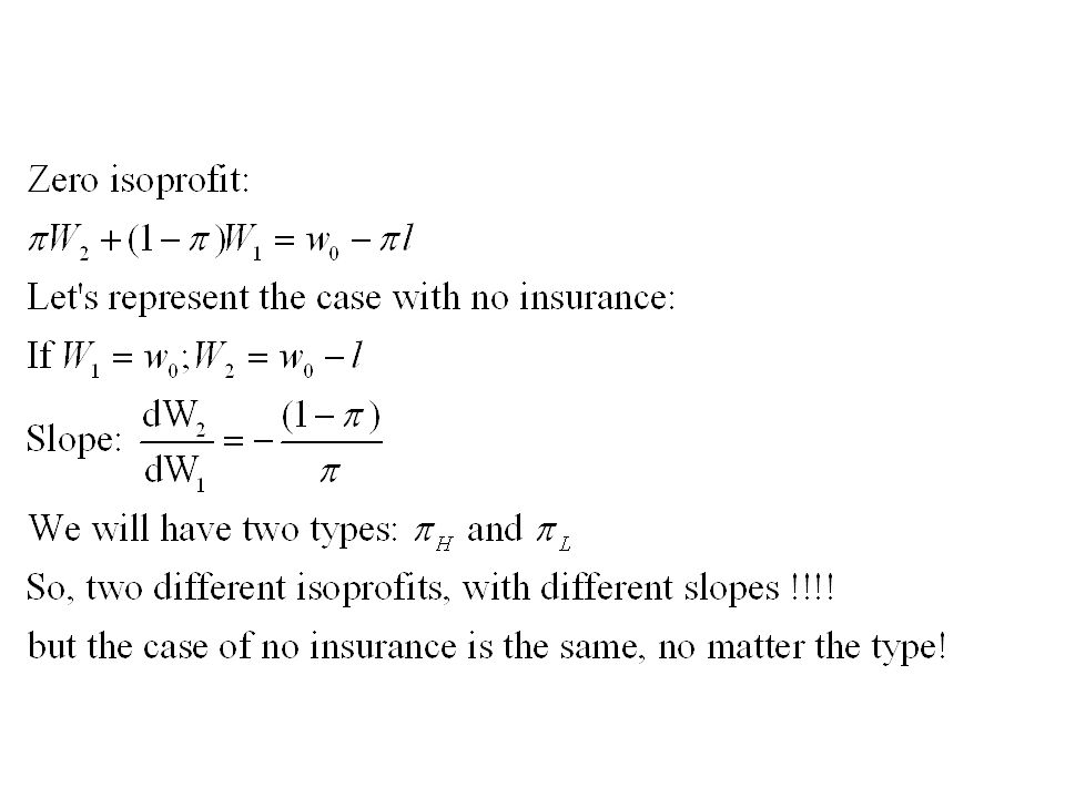
31. E=Point of no insuranceW2
certainty line
W 0
W0*- l
E=Point of no insurance E W1

32. The low-risk person will maximize utility at point
certainty line F G
The low-risk person will
maximize utility at point
F, while the high-risk
person will choose G
W 0 - l E W1
W 0

33. Draw the indifference curves to show the equilibrium under symmetric information.
Notice the tangency between the indifference curve and the isoprofit in the certainity line W2
certainty line F G
The low-risk person will
maximize utility at point
F, while the high-risk
person will choose G
W 0 - l E W1
W 0

34. Adverse Selection
If insurers have imperfect information about which individuals fall into low- and high-risk categories, this solution is unstable
point F provides more wealth in both states
high-risk individuals will want to buy insurance that is intended for low-risk individuals
insurers will lose money on each policy sold

35. Adverse Selection
One possible solution would be for the insurer to offer premiums based on the average probability of loss H W2
certainty line F
Since EH does not
accurately reflect the true
probabilities of each buyer,
they may not fully insure
and may choose a point
such as M M G
W0 - l E W1
W 0

36. Adverse Selection
Point M (which is a pooling candidate) is not an equilibrium because further trading
opportunities exist for low-risk individuals UH UL W2
certainty line
An insurance policy
such as N would be
unattractive to high-
risk individuals, but
attractive to low-risk
individuals and
profitable for insurers N F H M G
W 0 - l E W1 W0

37. Adverse Selection
If a market has asymmetric information, the equilibria must be separated in some way
high-risk individuals must have an incentive to purchase one type of insurance, while low-risk purchase another

38. Adverse Selection
Suppose that insurers offer policy G. High-risk individuals will opt for full insurance. UH W2
certainty line
Insurers cannot offer any policy that lies above UH because
they cannot prevent high-risk individuals from taking advantage of it F G
W0 - l E W1
W 0

39. Adverse Selection
The best policy that low-risk individuals can obtain is one such as J J W2
certainty line F
The policies G and J
represent a separating equilibrium UH G
W * - l E W1
W *

40. Adverse Selection
The policies G and J represent a separating equilibrium. Notice that the Low risk only gets an INCOMPLETE insurance. So, we can have results that depend on outcomes even if there is no moral hazard!!!! J W2
certainty line F UH G
W * - l E W1
W *

41. Parallelisms… Workers model SI: If offered under AI:
High constant wage for G type (productive)
Low constant wage for B type (unproductive)
If offered under AI:
Type B will pass himself off as G type
Type B has “something to sell”
Insurance companies:
SI:
-Full ins. with low premium for G type (low p. ac.)
-Full ins. with high premium for B type (high p. of ac.)
If offered under AI:
Type B will pass himself off as G type
Type B has “something to sell”

42. Parallelisms… Workers model AS: Insurance companies: AS:
Type B has “something to sell”
AS:
B: fixed wage: full ins. Same contract as under SI
G: no full insurance. Distorted contract. Worse off due to AS
Insurance companies:
Type B has “something to sell”
AS:
B (high prob. acc): full ins. Same contract as under SI
G (low prob. acc): no full insurance. Distorted contract. Worse off due to AS !!!
We can see how it is the type with low probability of accident the one that ends up having incomplete insurance !! It is the one worse off due to AS !!!!

43. Insurance contracts
Menu of contracts: one with full insurance, another one with incomplete insurance.
This is what we observe in reality with most types of insurance contracts (car, health…)
Insurance contracts usually have an “excess”. But the “excess” can be eliminated by paying an additional premium
Insurance excess (from this link) Applies to an insurance claim and is simply the first part of any claim that must be covered by yourself. This can range from £50 to £1000 or higher. Increasing your excess can significantly reduce your premium. On the other hand a waiver can sometimes be paid to eliminate any excess at all.