Download presentation
Presentation is loading. Please wait.

1
Multivariate Description

2
What Technique? Response variable(s)... Predictors(s) No Predictors(s) Yes... is one distribution summary regression models... are many indirect gradient analysis (PCA, CA, DCA, MDS) cluster analysis direct gradient analysis constrained cluster analysis discriminant analysis (CVA)
 cluster analysis direct gradient analysis constrained cluster analysis discriminant analysis (CVA).")
3
a) Rotate the Variable Space
 Rotate the Variable Space")
4
Raw Data

5
Linear Regression

6
Two Regressions

7
Principal Components

8
Gulls Variables

9
Scree Plot

10
Output > gulls.pca2$loadings Loadings: Comp.1 Comp.2 Comp.3 Comp.4 Weight -0.505 -0.343 0.285 0.739 Wing -0.490 0.852 -0.143 0.116 Bill -0.500 -0.381 -0.742 -0.232 H.and.B -0.505 -0.107 0.589 -0.622 > summary(gulls.pca2) Importance of components: Comp.1 Comp.2 Comp.3 Standard deviation 1.8133342 0.52544623 0.47501980 Proportion of Variance 0.8243224 0.06921464 0.05656722 Cumulative Proportion 0.8243224 0.89353703 0.95010425
 Importance of components: Comp.1 Comp.2 Comp.3 Standard deviation Proportion of Variance Cumulative Proportion")
11
Bi-Plot

12
Male or Female?

13
Linear Discriminant > gulls.lda <- lda(Sex ~ Wing + Weight + H.and.B + Bill, gulls) lda(Sex ~ Wing + Weight + H.and.B + Bill, data = gulls) Prior probabilities of groups: 0 1 0.5801105 0.4198895 Group means: Wing Weight H.and.B Bill 0 410.0381 871.7619 115.1143 17.62524 1 430.6118 1054.3092 125.9474 19.50789 Coefficients of linear discriminants: LD1 Wing 0.045512619 Weight 0.001887236 H.and.B 0.138127194 Bill 0.444847743
 lda(Sex ~ Wing + Weight + H.and.B + Bill, data = gulls) Prior probabilities of groups: Group means: Wing Weight H.and.B Bill Coefficients of linear discriminants: LD1 Wing Weight H.and.B Bill")
14
Discriminating

15
Relationship between PCA and LDA

16
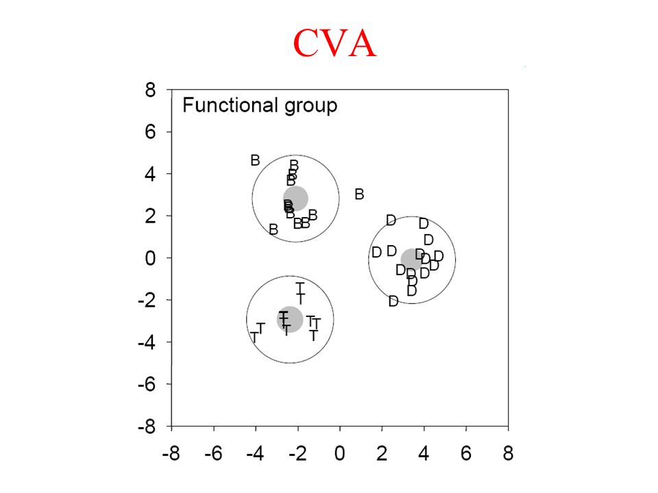
CVA

18
b) Use Distance or Dissimilarity (Multi-Dimensional Scaling)
 Use Distance or Dissimilarity (Multi-Dimensional Scaling)")
19
A Distance Matrix

20
Uses of Distances Distance/Dissimilarity can be used to:- Explore dimensionality in data (using PCO) As a basis for clustering/classification
 As a basis for clustering/classification")
21
UK Wet Deposition Network

22
Fitting Environmental Variables

23
A Map based on Measured Variables

24
Fitting Environmental Variables

25
c) Summarise by Weighted Averages
 Summarise by Weighted Averages")
26
Species and Sites as Weighted Averages of each other SITES 1 1 1111 1 2111 SPP. 23466185750198304927 Bel per 3.2....2..2..22..... Jun buf.3..........4..…42.. Jun art...3..4..3..4..4.... Air pra........2........3.. Ele pal...8..4..5.....44... Rum ace....6..5....2..…23.. Vic lat..........12.1...... Bra rut..246.22.4242624.342 Ran fla.2.2..2..2.....42... Hyp rad........2..2.....5.. Leo aut 522.3.33223525222623 Pot pal.........2......2... Poa pra 424.34421.44435.…4.. Cal cus...3...........34... Tri pra....5..2........…2.. Tri rep 521.5.22.163322.6232 Ant odo....3..44.4......4.2 Sal rep.............3.5.3.. Ach mil 3...21.22.4.....…2.. Poa tri 79524246..4.5.6…45.. Ely rep 4.4..4.4....6.4..... Sag pro.25...2....22....34. Pla lan....5..52.33.3..…5.. Agr sto.587..4..4..3.454.4. Lol per 5.5.6742..67226.…6.. Alo gen 2524..5.....3.7...8. Bro hor 4.3....2..4.....…2..

27
Species and Sites as Weighted Averages of each other

28
Reciprocal Averaging - unimodal Site A B C D E F Species Prunus serotina 6 3 4 6 5 1 Tilia americana 2 0 7 0 6 6 Acer saccharum 0 0 8 0 4 9 Quercus velutina 0 8 0 8 0 0 Juglans nigra 3 2 3 0 6 0

29
Reciprocal Averaging - unimodal Site A B C D E F Species Score Species Iteration 1 Prunus serotina 6 3 4 6 5 1 1.00 Tilia americana 2 0 7 0 6 6 0.63 Acer saccharum 0 0 8 0 4 9 0.63 Quercus velutina 0 8 0 8 0 0 0.18 Juglans nigra 3 2 3 0 6 0 0.00 Iteration 1 1.00 0.00 0.86 0.60 0.62 0.99 Site Score

30
Reciprocal Averaging - unimodal Site A B C D E F Species Score Species Iteration 1 2 Prunus serotina 6 3 4 6 5 1 1.00 0.68 Tilia americana 2 0 7 0 6 6 0.63 0.84 Acer saccharum 0 0 8 0 4 9 0.63 0.87 Quercus velutina 0 8 0 8 0 0 0.18 0.30 Juglans nigra 3 2 3 0 6 0 0.00 0.67 Iteration 1 1.00 0.00 0.86 0.60 0.62 0.99 Site 2 0.65 0.00 0.88 0.05 0.78 1.00 Score

31
Reciprocal Averaging - unimodal Site A B C D E F Species Score Species Iteration 1 2 3 Prunus serotina 6 3 4 6 5 1 1.00 0.68 0.50 Tilia americana 2 0 7 0 6 6 0.63 0.84 0.86 Acer saccharum 0 0 8 0 4 9 0.63 0.87 0.91 Quercus velutina 0 8 0 8 0 0 0.18 0.30 0.02 Juglans nigra 3 2 3 0 6 0 0.00 0.67 0.66 Iteration 1 1.00 0.00 0.86 0.60 0.62 0.99 Site 2 0.65 0.00 0.88 0.05 0.78 1.00 Score 3 0.60 0.01 0.87 0.00 0.78 1.00

32
Reciprocal Averaging - unimodal Site A B C D E F Species Score Species Iteration 1 2 3 9 Prunus serotina 6 3 4 6 5 1 1.00 0.68 0.50 0.48 Tilia americana 2 0 7 0 6 6 0.63 0.84 0.86 0.85 Acer saccharum 0 0 8 0 4 9 0.63 0.87 0.91 0.91 Quercus velutina 0 8 0 8 0 0 0.18 0.30 0.02 0.00 Juglans nigra 3 2 3 0 6 0 0.00 0.67 0.66 0.65 Iteration 1 1.00 0.00 0.86 0.60 0.62 0.99 Site 2 0.65 0.00 0.88 0.05 0.78 1.00 Score 3 0.60 0.01 0.87 0.00 0.78 1.00 9 0.59 0.01 0.87 0.00 0.78 1.00

33
Reordered Sites and Species Site A C E B D F Species Species Score Quercus velutina 8 8 0 0 0 0 0.004 Prunus serotina 6 3 6 5 4 1 0.477 Juglans nigra 0 2 3 6 3 0 0.647 Tilia americana 0 0 2 6 7 6 0.845 Acer saccharum 0 0 0 4 8 9 0.909 Site Score 0.000 0.008 0.589 0.778 0.872 1.000

34
Managing Dimensionality (but not acronyms) PCA, CA, RDA, CCA, MDS, NMDS, DCA, DCCA, pRDA, pCCA
 PCA, CA, RDA, CCA, MDS, NMDS, DCA, DCCA, pRDA, pCCA")
35
Type of Data Matrix species sites attributes species attributes sites attributes individuals desert macroph inverts uses watervar rain gulls

36
Ordination Techniques Linear methodsWeighted averaging unconstrainedPrincipal Components Analysis (PCA) Correspondence Analysis (CA) constrainedRedundancy Analysis (RDA) Canonical Correspondence Analysis (CCA)
 Correspondence Analysis (CA) constrainedRedundancy Analysis (RDA) Canonical Correspondence Analysis (CCA)")
37
Models of Species Response There are (at least) two models:- Linear - species increase or decrease along the environmental gradient Unimodal - species rise to a peak somewhere along the environmental gradient and then fall again
 two models:- Linear - species increase or decrease along the environmental gradient Unimodal - species rise to a peak somewhere along the environmental gradient and then fall again")
38
A Theoretical Model

39
Linear

40
Unimodal

41
Alpha and Beta Diversity alpha diversity is the diversity of a community (either measured in terms of a diversity index or species richness) beta diversity (also known as species turnover or differentiation diversity) is the rate of change in species composition from one community to another along gradients; gamma diversity is the diversity of a region or a landscape.
 beta diversity (also known as species turnover or differentiation diversity) is the rate of change in species composition from one community to another along gradients; gamma diversity is the diversity of a region or a landscape.")
42
A Short Coenocline

43
A Long Coenocline

44
Inferring Gradients from Species (or Attribute) Data
 Data")
45
Indirect Gradient Analysis Environmental gradients are inferred from species data alone Three methods: –Principal Component Analysis - linear model –Correspondence Analysis - unimodal model –Detrended CA - modified unimodal model

46
PCA - linear model

48
Terschelling Dune Data

49
PCA gradient - site plot

50
PCA gradient - site/species biplot standard nature biodynamic & hobby

51
Arches - Artifact or Feature?

52
The Arch Effect What is it? Why does it happen? What should we do about it?

53
From Alexandria to Suez

54
CA - with arch effect (sites)
")
55
CA - with arch effect (species)
")
56
Long Gradients ABCD

57
Gradient End Compression

58
CA - with arch effect (species)
")
59
CA - with arch effect (sites)
")
60
Detrending by Segments

61
DCA - modified unimodal

62
Making Effective Use of Environmental Variables

63
Approaches Use single responses in linear models of environmental variables Use axes of a multivariate dimension reduction technique as responses in linear models of environmental variables Constrain the multivariate dimension reduction into the factor space defined by the environmental variables

64
Unconstrained/Constrained Unconstrained ordination axes correspond to the directions of the greatest variability within the data set. Constrained ordination axes correspond to the directions of the greatest variability of the data set that can be explained by the environmental variables.

65
Direct Gradient Analysis Environmental gradients are constructed from the relationship between species environmental variables Three methods: –Redundancy Analysis - linear model –Canonical (or Constrained) Correspondence Analysis - unimodal model –Detrended CCA - modified unimodal model
 Correspondence Analysis - unimodal model –Detrended CCA - modified unimodal model")
66
Direct Gradient Analysis Basic PCA y ik = b 0k + b 1k x i + e ik –x i - the sample scores on the ordination axis –b 1k - the regression coefficients for each species (the species scores on the ordination axis) In RDA there is a further constraint on x i x i = c 1 z i1 + c 2 z i2 Making y ik = b 0k + b 1k c 1 z i1 + b 1k c 2 z i2 + e ik
 In RDA there is a further constraint on x i x i = c 1 z i1 + c 2 z i2 Making y ik = b 0k + b 1k c 1 z i1 + b 1k c 2 z i2 + e ik")
67
Direct Gradient Analysis cca(species_data ~ e1 + e2 +... + en + Condition(e5), data=environmental_data) cca(varespec ~ Al + P*(K + Baresoil) + Condition(pH), data=varechem)
, data=environmental_data) cca(varespec ~ Al + P*(K + Baresoil) + Condition(pH), data=varechem).")
68
Lake Nasser - Egypt

69
CCA - site/species joint plot

70
CCA - species/environment biplot

71
Removing the Effect of Nuisance Variables

72
Partial Analyses Remove the effect of covariates –variables that we can measure but which are of no interest –e.g. block effects, start values, etc. Carry out the gradient analysis on what is left of the variation after removing the effect of the covariates.

73
Cluster Analysis

74
Different types of data example Continuous data:height Categorical data ordered (nominal):growth rate very slow, slow, medium, fast, very fast not ordered:fruit colour yellow, green, purple, red, orange Binary data:fruit / no fruit
:growth rate very slow, slow, medium, fast, very fast not ordered:fruit colour yellow, green, purple, red, orange Binary data:fruit / no fruit")
75
Similarity matrix We define a similarity between units – like the correlation between continuous variables. (also can be a dissimilarity or distance matrix) A similarity can be constructed as an average of the similarities between the units on each variable. (can use weighted average) This provides a way of combining different types of variables.
 A similarity can be constructed as an average of the similarities between the units on each variable. (can use weighted average) This provides a way of combining different types of variables..")
76
relevant for continuous variables: Euclidean city block or Manhattan Distance metrics A B A B (also many other variations)
")
77
Similarity coefficients for binary data simple matching count if both units 0 or both units 1 Jaccard count only if both units 1 (also many other variants) simple matching can be extended to categorical data 0,11,1 0,01,0 0,11,1 0,01,0
 simple matching can be extended to categorical data 0,11,1 0,01,0 0,11,1 0,01,0")
78
hierarchical divisive put everything together and split monothetic / polythetic agglomerative keep everything separate and join the most similar points (classical cluster analysis) non-hierarchical k-means clustering Clustering methods
 non-hierarchical k-means clustering Clustering methods")
79
Agglomerative hierarchical Single linkage or nearest neighbour finds the minimum spanning tree: shortest tree that connects all points chaining can be a problem

80
Agglomerative hierarchical Complete linkage or furthest neighbour compact clusters of approximately equal size. (makes compact groups even when none exist)
.")
81
Agglomerative hierarchical Average linkage methods between single and complete linkage

82
Testing Significance in Ordination

83
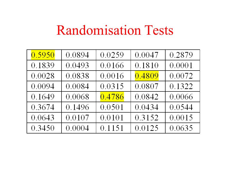
Randomisation Tests

85
Randomisation Example Model: cca(formula = dune ~ Moisture + A1 + Management, data = dune.env) Df Chisq F N.Perm Pr(>F) Model 7 1.1392 2.0007 200 < 0.005 *** Residual 12 0.9761 Signif. codes: 0 *** 0.001 ** 0.01 * 0.05

Similar presentations


 PCA, CA, RDA, CCA, MDS, NMDS, DCA, DCCA, pRDA, pCCA.>")

... Predictors(s) No Predictors(s) Yes... is one distribution summary regression models...>")
... Predictors(s) No Predictors(s) Yes... is one distribution summary regression models...>")


... Predictors(s) No Predictors(s) Yes... is one distribution summary regression models...>")
 Tom Price 3 March 2009.>")


>")
 www.talksport.co.uk Nick Korach UP-STAT 2013.>")


 Shan March 3, 2015 LISA: Multivariate Analysis in RMar. 3, 2015.>")

